Visualization

`trueq.visualization.multiply_lightness`	Modifies a color by multiplying `(1 - lightness)` in HSL space by the given amount.
`trueq.visualization.plot_mat`	Plot a complex matrix with labeling.
`trueq.visualization.plot_results`	Generates a bar chart plot for one or multiple `Results` objects using a variety of user-specified plotting styles.
`trueq.visualization.plotters.PlottingSuite`	A collection of `Plotter`s, which are accessible as methods of instances of this class.
`trueq.visualization.plotters.abstract.Plotter`	Represents a function that performs a plotting operation either on a `EstimateCollection` or a `CircuitCollection` (with data).
`trueq.visualization.plotters.comparisons.compare`	A very generic plotter that compares like estimates across a specified key keyword.
`trueq.visualization.plotters.comparisons.compare_pauli_infidelities`	Plotter that compares Pauli infidelities from CB, SC, and KNR.
`trueq.visualization.plotters.comparisons.compare_rb`	Compares SRB and XRB infidelities vs twirling groups.
`trueq.visualization.plotters.comparisons.compare_twirl`	Very generic plotter that compares like estimates across subsystems of a multi-system register.
`trueq.visualization.plotters.irb.irb_summary`	Plots estimate fits from IRB.
`trueq.visualization.plotters.mitigation.raw_nox`	Plots the estimates of the individual NOX circuits alongside the mitigated estimates.
`trueq.visualization.plotters.nr.knr_heatmap`	Plots KNR data as a heatmap.
`trueq.visualization.plotters.raw.raw`	Very generic plotter that overlays exponential fits onto lightly processed data.
`trueq.visualization.plotters.timestamps.timestamps`	Plots the timestamps of circuit results.
`trueq.visualization.Graph`	Represents a planar embedding of a quantum device seen as a graph.

Graph

class trueq.visualization.Graph(locations, edges=None, show_labels=False, bounds=None, mapping=None)

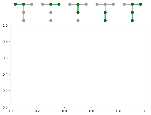
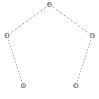
Represents a planar embedding of a quantum device seen as a graph.

The nodes of the graph represent qubits and the edges are possible couplings. The purpose of this class is to draw this graph in figures.

import trueq as tq
import matplotlib.pyplot as plt

g = tq.visualization.Graph(
    {0: (0.1, 0.9), 1: (0.5, 0.9), 2: (0.9, 0.9), 3: (0.5, 0.5), 4: (0.5, 0.1)},
    [[0, 1], [1, 2], [1, 3], [3, 4]],
)

plt.figure()
ax = plt.subplot()

cycles = [
    tq.Cycle({(0, 1): tq.Gate.cx}),
    tq.Cycle({(1, 2): tq.Gate.cx}),
    tq.Cycle({(1, 3): tq.Gate.cx}),
    tq.Cycle({(3, 4): tq.Gate.cx}),
    tq.Cycle({(1, 2): tq.Gate.cx, (3, 4): tq.Gate.cx}),
]

for idx, cycle in enumerate(cycles):
    g.add_graph(ax, (0.1 + 0.2 * idx, 1.03), width=0.15, cycle=cycle)

# save_figure may not catch things outside of the axis without this
plt.tight_layout()

Note

There are a number of class variable such as NODE_SIZE which can be altered on a given instance to change the properties of the displayed graph.

Parameters:

locations (dict) – A dictionary mapping qubit labels to locations. The locations should fall inside the unit square; they are scaled to the appropriate size when add_graph() is called. The argument bounds can be modified if it is more convenient to specify them in another box.
edges (Iterable) – A list of length-2 tuples specifying the allowed edges.
show_labels (bool | str) – Whether to display qubit label numbers (True), their mapped values based on mapping ("mapped"), or none at all (False) on the qubit nodes. Their properties can be adjusted by modifying the class variables LABEL_OFFSET, LABEL_STYLE, and LABEL_REPR.
bounds (tuple) – A tuple (left, right, bottom, top) indicating the drawing area extents of the coordinates in locations. By default, this is (0, 0, 1, 1).
mapping (dict) – A dictionary specifying how qubit labels can be mapped to some other convention. The values of this dictionary are shown on plotted graphs if show_labels=="mapped".

NODE_COLOR = '#999999': The color of a node.

NODE_SIZE = 4: The radius of a node in points.

ACTIVE_NODE_COLOR = (0.12423529411764711, 0.34635294117647064, 0.1863529411764707): The color of a node if a given cycle has a single-qubit gate acting on it.

LABELED_NODE_DIAMETER = 7: The radius of a node if show_labels is true.

EDGE_COLOR = '#999999': The color of an edge.

EDGE_WIDTH = 1: The width of an edge in points.

ACTIVE_EDGE_COLOR = '#42b863': The color of an edge if a given cycle has a two-qubit gate acting on it.

ACTIVE_EDGE_FRAC = 1: The width of an edge as a fraction of node radius.

LABEL_OFFSET = (0, 0): The offset of a node label in the same units as locations

LABEL_REPR: alias of str

LABEL_STYLE = {'color': 'w', 'fontsize': 11, 'ha': 'center', 'va': 'center', 'weight': 'bold'}: Text style properties to draw labels with.

property edges

A tuple of edges contained in this Graph.

import trueq as tq

tq.visualization.Graph.linear(5).edges

(frozenset({3, 4}), frozenset({0, 1}), frozenset({2, 3}), frozenset({1, 2}))

Type:: tuple

property labels

The sorted system labels in this Graph.

import trueq as tq

tq.visualization.Graph.linear(5).edges

(frozenset({3, 4}), frozenset({0, 1}), frozenset({2, 3}), frozenset({1, 2}))

Type:: tuple

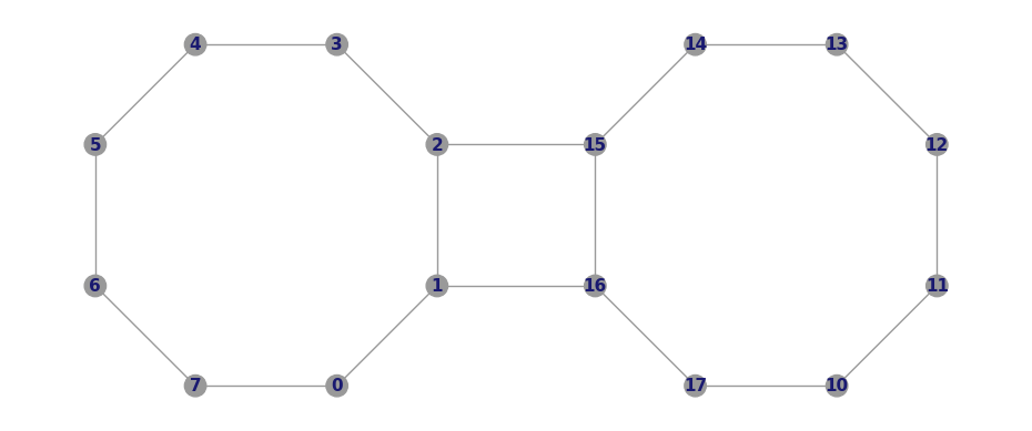
aspen_11()

Instantiates a new Graph with a 38 qubit topology found on the Rigetti Aspen-11 chip.

import trueq as tq

tq.visualization.Graph.aspen_11(show_labels=True).plot()

Parameters:: show_labels (bool) – Whether to display qubit label numbers on the qubit nodes.
Return type:: Graph

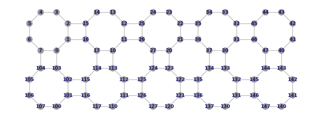
aspen_m_1()

Instantiates a new Graph with an 80 qubit topology found on the Rigetti Aspen-M-1 chip.

import trueq as tq

g = tq.visualization.Graph.aspen_m_1(show_labels=True)
g.LABEL_STYLE["color"] = "midnightblue"
g.plot()

Parameters:: show_labels (bool) – Whether to display qubit label numbers on the qubit nodes.
Return type:: Graph

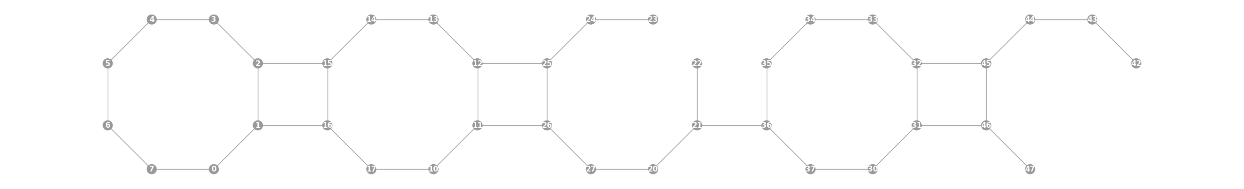
rigetti_octagon(n_cols, show_labels=False, omit=None)

Instantiates a new Graph where qubits are placed on a n_rows-by-n_cols grid of octagons, where each octagon of eight qubits is connected to each of its neighbouring octagons with two edges.

import trueq as tq

g = tq.visualization.Graph.rigetti_octagon(1, 2, show_labels=True)
g.LABEL_STYLE["color"] = "midnightblue"
g.plot()

Parameters:

n_rows (int) – The number of rows of octagons.
n_cols (int) – The number of columns of octagons.
show_labels (bool) – Whether to display qubit label numbers on the qubit nodes.
omit (int | Iterable) – An iterable of labels or edges to omit from the graph. For example, (2, 3, 5) will omit qubits 2, 3, and 5 from the graph along with incident edges, whereas (2, (3, 5)) will omit qubit 2 as well as edge (3, 5) although qubits 3 and 5 will still be present.

Return type:

Graph

static ibmq_grid(rows, row_major=True, show_labels=False)

Convenience constructor for qubits that lie on a sparse grid of a form particularly popular with IBMQ devices. Each element of rows should be a length-4 list with entries (n_qubits, offset, links, n_int) where

n_qubits is the number of qubits in the row, all connected as a chain.

offset is the integer horizontal offset of the row from 0.

links is a list of positions in the row at which to add vertical links.

n_int is the number of extra qubits to add in each vertical link.

import trueq as tq

# create topology shared by Paris, Montreal, and Toronto IBMQ chips,
# equivalent to calling Graph.ibmq_27()
# note that the 0-qubit first row is used to create the top vertical links
g = tq.visualization.Graph.ibmq_grid(
    [(0, 0, [3, 7], 1), (10, 0, [1, 5, 9], 1), (10, 1, [2, 6], 1)],
    row_major=False,
    show_labels=True,
)
g.plot()

Parameters:

rows (list) – A list of lists as described above:
row_major (bool) – Whether qubit labels should increment left-to-right-top-to-bottom (True) or top-to-bottom-left-to-right (False).
show_labels (bool) – Whether to display qubit label numbers on the qubit nodes.

Return type:

Graph

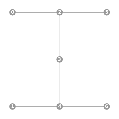
static ibmq_7(show_labels=False)

Instantiates a new Graph with a 7 qubit topology found on some IBMQ devices (including the “Lagos”, “Oslo”, “Nairobi”, and “Perth” chips).

import trueq as tq

tq.visualization.Graph.ibmq_7(show_labels=True).plot()

Parameters:: show_labels (bool) – Whether to display qubit label numbers on the qubit nodes.
Return type:: Graph

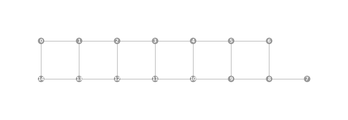
static ibmq_15(show_labels=False)

Instantiates a new Graph with a 15 qubit topology found on some IBMQ devices (including the “Melbourne” chip).

import trueq as tq

tq.visualization.Graph.ibmq_15(show_labels=True).plot()

Parameters:: show_labels (bool) – Whether to display qubit label numbers on the qubit nodes.
Return type:: Graph

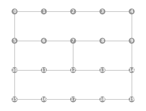
static ibmq_20a(show_labels=False)

Instantiates a new Graph with a 20 qubit topology found on some IBMQ devices (including the “Almaden”, “Boeblingen”, and “Singapore” chips).

import trueq as tq

tq.visualization.Graph.ibmq_20a(show_labels=True).plot()

Parameters:: show_labels (bool) – Whether to display qubit label numbers on the qubit nodes.
Return type:: Graph

static ibmq_20b(show_labels=False)

Instantiates a new Graph with a 20 qubit topology found on some IBMQ devices (including the “Johannesburg” and “Poughkeepsie” chips).

import trueq as tq

tq.visualization.Graph.ibmq_20b(show_labels=True).plot()

Parameters:: show_labels (bool) – Whether to display qubit label numbers on the qubit nodes.
Return type:: Graph

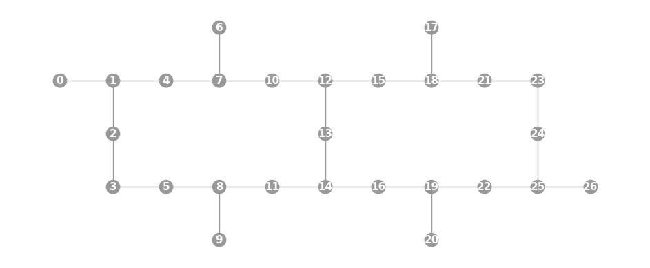
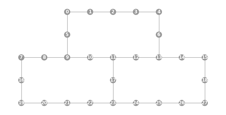
static ibmq_27(show_labels=False)

Instantiates a new Graph with a 27 qubit topology found on some IBMQ devices (including the “Montreal”, “Paris”, and “Toronto” chips).

import trueq as tq

tq.visualization.Graph.ibmq_27(show_labels=True).plot()

Parameters:: show_labels (bool) – Whether to display qubit label numbers on the qubit nodes.
Return type:: Graph

static ibmq_28(show_labels=False)

Instantiates a new Graph with a 28 qubit topology found on some IBMQ devices (including the “Cambridge” chip).

import trueq as tq

tq.visualization.Graph.ibmq_28(show_labels=True).plot()

Parameters:: show_labels (bool) – Whether to display qubit label numbers on the qubit nodes.
Return type:: Graph

static ibmq_53(show_labels=False)

Instantiates a new Graph with a 53 qubit topology found on some IBMQ devices (including the “Rochester” chip).

import trueq as tq

tq.visualization.Graph.ibmq_53(show_labels=True).plot()

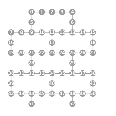
Parameters:: show_labels (bool) – Whether to display qubit label numbers on the qubit nodes.
Return type:: Graph

static ibmq_65(show_labels=False)

Instantiates a new Graph with a 65 qubit topology found on some IBMQ devices (including the “Manhattan” chip).

import trueq as tq

tq.visualization.Graph.ibmq_65(show_labels=True).plot()

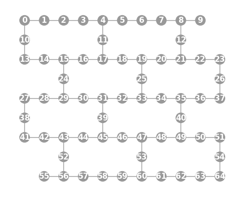
Parameters:: show_labels (bool) – Whether to display qubit label numbers on the qubit nodes.
Return type:: Graph

static ibmq_butterfly(show_labels=False)

Instantiates a new Graph with a butterfly-shaped 5 qubit topology found on some IBMQ devices (including the “Yorktown” chip).

import trueq as tq

tq.visualization.Graph.ibmq_butterfly(show_labels=True).plot()

Parameters:: show_labels (bool) – Whether to display qubit label numbers on the qubit nodes.
Return type:: Graph

static ibmq_T(show_labels=False)

Instantiates a new Graph with a T-shaped 5 qubit topology found on some IBMQ devices (including the “Ourense”, “Vigo”, and “Valencia” chips).

import trueq as tq

tq.visualization.Graph.ibmq_T(show_labels=True).plot()

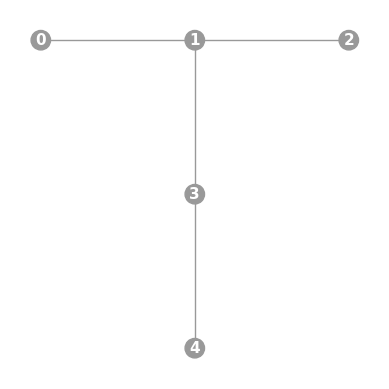
Parameters:: show_labels (bool) – Whether to display qubit label numbers on the qubit nodes.
Return type:: Graph

static linear(n, show_labels=False)

Instantiates a new Graph with a linear topology.

To condense the size of the displayed graph, nodes are placed on a circle.

import trueq as tq

tq.visualization.Graph.linear(5, show_labels=True).plot()

Parameters:

n (int | Iterable) – The number of qubits or an iterable of qubit labels.
show_labels (bool) – Whether to display qubit label numbers on the qubit nodes.

Return type:

Graph

grid(n_cols, show_labels=False)

Instantiates a new Graph with a grid topology.

Qubit labels start at 0 and are rastered left-to-right from the top-left of the grid.

import trueq as tq

tq.visualization.Graph.grid(3, 4, show_labels=True).plot()

Parameters:

n_rows (int) – The number rows in the grid.
n_cols (int) – The number columns in the grid.
show_labels (bool | bool) – Whether to display qubit label numbers on the qubit nodes (True), the labeled coordinate ("mapped"), or no label (False).

Return type:

Graph

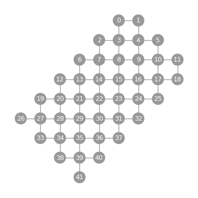
static sycamore(n_rows, n_cols, show_labels=False)

Instantiates a new Graph with a diagonal grid topology.

Qubit labels are ordered by qubit position sorted with row-major ordering, where the origin is taken as the top left of the embedding.

import trueq as tq

tq.visualization.Graph.sycamore(7, 6, show_labels=True).plot()

Parameters:

n_rows (int) – The number of rows if the grid were rotated 45 degrees clockwise.
n_cols (int) – The number of (zig-zagging) columns if the grid were rotated 45 degrees clockwise.
show_labels (bool | bool) – Whether to display qubit label numbers on the qubit nodes (True), the labeled coordinate ("mapped"), or no label (False).

Return type:

Graph

to_label(val)

Converts some value to a qubit label.

Parameters:: val – Some valid value specified in the constructor’s mapping argument.
Return type:: int
Raises:: KeyError – If val is unknown.

from_label(label)

Converts some qubit label to the value specified by the construtor’s mapping argument.

Parameters:: label (int) – A qubit label.
Return type:: int
Raises:: KeyError – If label is not in this graph.

add_graph(ax, xy, cycle=None, twirl=None, transform=None, width=None, height=None, xorigin='center', yorigin='bottom', aspect=None)

Embeds the graph into a matplotlib axis at a given position and size.

Certain edges of the graph can be highlighted by passing a cycle.

Parameters:

ax (matplotlib.artist.Artist) – The axis (or any other type of artist) to add the graph to.
xy (tuple) – The x and y position at which to add the graph, in coordinates specified by transform.
cycle (trueq.Cycle) – Coupled edges and active nodes in this cycle will be highlighted in the graph.
twirl (tuple) – Twirled edges and nodes in the twirl will be highlighted in the graph.
transform (matplotlib.transforms.Transform) – Specifies the units of x, y, width and height. By default, takes the value blended_transform_factory(ax.transData, ax.transAxes) so that horizontal units are data units, and vertical units are axis units.
width (float) – The width graph, in coordinates specified by transform. This is optional, see aspect for details.
height (float) – The width graph, in coordinates specified by transform. This is optional, see aspect for details.
xorigin (str | float) – One of "left", "center", “right”, or any value between 0 and 1. Specifies which point of the graph’s bounding box should be located at position x.
yorigin (str | float) – One of “bottom”, “middle”, “top”, or any value between 0 and 1. Specifies which point of the graph’s bounding box should be located at position `y.
aspect (float) – Force a display aspect ratio of the graph’s bounding box. This is done by computing the largest rectangle of the given aspect ratio that fits in the rectangle of size (width, height). By default, if both width and height are provided, then these numbers (after being converted to display units) define the aspect ratio. However, if only one of width or height are given, then a default aspect ratio is defined as the aspect ratio of the bounds set at initialization (default is 1).

plot(cycle=None, twirl=None)

Plots the graph in its own figure.

Parameters:

cycle (trueq.Cycle) – Coupled edges and active nodes in this cycle will be highlighted in the graph.
twirl (tuple) – Twirled edges and nodes in the twirl will be highlighted in the graph.

Multipy Lightness

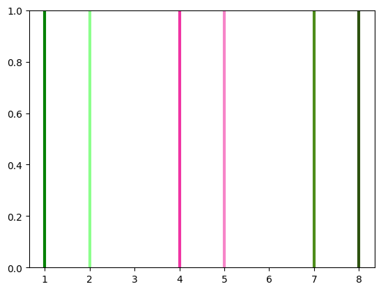
trueq.visualization.multiply_lightness(color, amount=0.5)

Modifies a color by multiplying (1 - lightness) in HSL space by the given amount.

Numbers less than 1 result in a lighter color, and numbers greater than 1 result in a darker color.

from trueq.visualization.general import multiply_lightness
import matplotlib.pyplot as plt

plt.axvline(1, lw=3, color="g")
plt.axvline(2, lw=3, color=multiply_lightness("g", 0.3))

plt.axvline(4, lw=3, color="#F034A3")
plt.axvline(5, lw=3, color=multiply_lightness("#F034A3", 0.6))

plt.axvline(7, lw=3, color=(0.3, 0.55, 0.1))
plt.axvline(8, lw=3, color=multiply_lightness((0.3, 0.55, 0.1), 1.2))

<matplotlib.lines.Line2D at 0x7f38d92b95e0>

Parameters:

color (str | tuple) – A matplotlib color string, hex string, or RGB tuple.
amount (float) – The amount to multiply (1 - lightness) of the input color by.

Returns:

An RGB tuple.

Return type:

tuple

Plot Mat

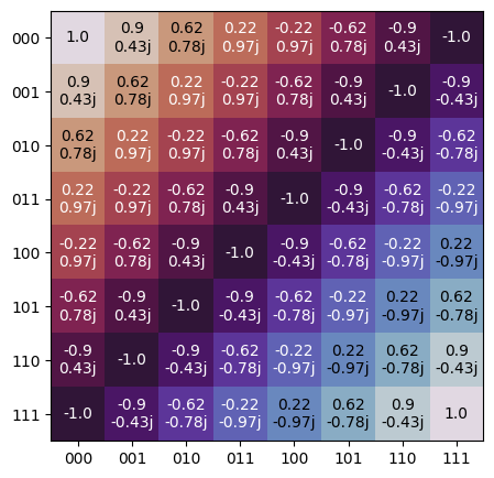
trueq.visualization.plot_mat(mat, xlabels=None, ylabels=None, show_values=True, abs_max=None, ax=None, xgrid=None, ygrid=None, blocks=None)

Plot a complex matrix with labeling.

The plot will have the following properties:

Color is dictated by the complex angle of each cell.
Transparency (alpha) is decided by the magnitude of each cell.
Size of plot scales based on shape of mat.

import trueq as tq
import numpy as np

phase = [np.exp(1j * t * np.pi) for t in np.linspace(0, 1, 8)]
tq.plot_mat(np.outer(phase, phase))

Parameters:

mat (numpy.ndarray-like) – A real or complex matrix.
xlabels (int | Iterable | NoneType) – Either None, an iterable of labels for the x-axis, or the dimension of the subsystems where the x-axis labels are the computational basis states as inferred from the size of mat. If None, the subsystem dimension will be inferred automatically.
ylabels (int | Iterable | NoneType) – Either None, an iterable of labels for the y-axis, or the dimension of the subsystems where the y-axis labels are the computational basis states as inferred from the size of mat. If None, the subsystem dimension will be inferred automatically.
show_values (bool) – Whether to show the numeric values of the matrix in each cell.
abs_max (NoneType | float) – The value to scale absolute values of the matrix by; the value at which plotted colors become fully opaque. By default, this is the largest absolute magnitude of the input matrix.
ax (matplotlib.Axis) – An existing axis to plot on. If not given, a new figure will be created.
xgrid (int | Iterable | NoneType) – An integer specifying the number of columns of separation between vertical grid lines, or a list of integers specifying all of the 0-indexed column numbers before which to place a grid line. If None, no vertical gridlines are placed.
ygrid (int | Iterable | NoneType) – An integer specifying the number of rows of separation between horizontal grid lines, or a list of integers specifying all of the 0-indexed row numbers before which to place a grid line. If None, no horizontal gridlines are placed.
blocks (Iterable | NoneType) – An iterable of members of the form ((i, j), (n_rows, n_cols)), where (i, j) are row and column indices of the matrix specifying the top-left position of a block, and where (n_rows, n_cols) are the number of rows and columns of the block. A rectangular outline will be drawn around each block. If None, no blocks will be drawn.

Plot Results

trueq.visualization.plot_results(*results, labels=None, normalize=None, sparse_cutoff=True, axis=None, style='adjacent', error_bars=False)

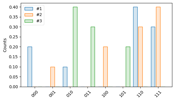
Generates a bar chart plot for one or multiple Results objects using a variety of user-specified plotting styles.

Valid style inputs are:

"adjacent": Results are plotted on the same graph next to each other

"overlay": Results are plotted on the same graph on top of each other

"separate": Results are plotted on a grid of separate axes

import trueq as tq
from trueq.visualization import plot_results

r1 = tq.Results({"000": 0.2, "010": 0.1, "110": 0.4, "111": 0.3})
r2 = tq.Results({"001": 0.1, "100": 0.2, "110": 0.3, "111": 0.4})
r3 = tq.Results({"011": 0.3, "010": 0.4, "101": 0.1, "101": 0.2})

plot_results(r1, r2, r3)

Note

A single Results can alternatively be plotted with the method plot().

If error_bars is set to True, then each bar on the plot that comes from a results object where n_shots is greater than 1 will have a shot-noise error bar attached to it. The size of these error bars are computed as follows. Suppose the \(i^\text{th}\) bitstring has \(y_i\) counts and comes from results with a total number of shots \(n\). Then we can consider the beta distribution \(\operatorname{Beta}(y_i, n-y_i)\) as the error of that particular bar, and we choose the extents of the error bar as the \(\alpha/2\) and \(1-\alpha/2\) percentiles of this distribution, where the confidence level \(\alpha\) is taken from get_cl(). The justification is that the Dirichlet distribution \(\operatorname{Dir}(y_1,\ldots,y_N)\) is the posterior distribution of the multinomial data \((y_1,\ldots,y_N)\) under the improper uninformative prior \(\operatorname{Dir}(0,\ldots,0)\), so that \(\operatorname{Beta}(y_i, n-y_i)\) is the posterior marginal distribution of index \(i\). These bounds are asymptotically equal to \(\pm z\sqrt{\frac{y_i}{n}(1-\frac{y_i}{n})/n}\) where \(z\) effects the normal confidence level \(\alpha\).

Parameters:

*results – One or more Results instances.
labels (Iterable | NoneType) – Either None or a list of string labels corresponding to the input results. If None, default labels will be applied to the plot.
normalize (NoneType | Bool) – Either None or a boolean value to specify whether results should be normalized for plotting. When None, results appearing on the same axis will all be normalized when their numbers of shots differ.
sparse_cutoff (Bool) – Boolean value to specify whether to clip small values.
axis (NoneType | matplotlib.pyplot.axis | Iterable) – Either None or a single or multiple matplotlib axis instances on which to plot the results.
style (str) – A string to specify the plot style. Valid options are "adjacent", "overlay" and "separate".
error_bars (bool) – Whether or not to plot shot-noise errorbars, as described above.

Raises:

ValueError – If no results were provided or if the results have different values of n_measurements.

Compare

class trueq.visualization.plotters.comparisons.compare

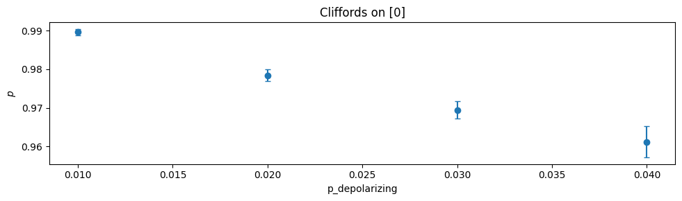
A very generic plotter that compares like estimates across a specified key keyword.

Note

This class typically should not be invoked directly by users; the main plotting method is exposed dynamically by the attributes trueq.CircuitCollection.plot and trueq.estimate.EstimateCollection.plot if relevant.

static plot(fit, names, keyword, label_rotation=0, axes=None, filename=None)

Plots a comparison of the value of one or more estimates specified by names versus the value of keyword found in each estimate’s key. Within each subplot, all other keywords and values are constant.

import trueq as tq

all_circuits = tq.CircuitCollection()
for p in [0.01, 0.02, 0.03, 0.04]:
    circuits = tq.make_srb(0, [4, 20, 40])
    tq.Simulator().add_depolarizing(p).run(circuits)
    all_circuits.append(circuits.update_keys(p_depolarizing=p))

all_circuits.plot.compare("p", "p_depolarizing")

Parameters:

fit (EstimateCollection | CircuitCollection) – A collection of circuits or their fit.
names (Iterable | str) – A name or a list of names specifying which estimate parameters should be included in the plot as y-values.
keyword (str) – A keyword found in the estimates’ keys whose values the given parameters will be compared against.
label_rotation (float) – The rotation of x-axis labels in degrees.
axes (Iterable) – An iterable of existing axes. If none are provided, new axes are created. Note that axis instances can be repeated in this list if you want to force the combination of subfigures that would normally be distinct, see axes() for an example.
filename (str) – An optional filename to save the file as. The extension determines the filetype; common choices are “.png”, “.pdf”, and “.svg”. If no extension is given, PNG is chosen.

Compare Pauli Infidelities

class trueq.visualization.plotters.comparisons.compare_pauli_infidelities

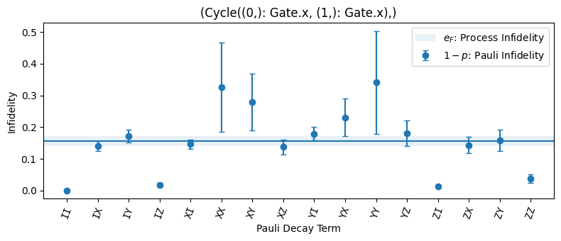
Plotter that compares Pauli infidelities from CB, SC, and KNR.

Note

This class typically should not be invoked directly by users; the main plotting method is exposed dynamically by the attributes trueq.CircuitCollection.plot and trueq.estimate.EstimateCollection.plot if relevant.

static plot(fit, graph=None, axis_size=(8, 3.5), axes=None, filename=None)

Plots a comparison of all Pauli infidelities measured by CB, KNR, or SCexperiments. In the case of SC, the process infidelity of the entire cycle, which is the average of all Pauli infidelities, is overlaid. Every unique experiment and sublabel combination is shown on a separate subplot.

import trueq as tq

circuits = tq.make_cb({0: tq.Gate.x, 1: tq.Gate.x}, [2, 8])
sim = tq.Simulator().add_stochastic_pauli(pz=0.04).add_overrotation(0.04)
sim.run(circuits)

circuits.plot.compare_pauli_infidelities()

Parameters:

fit (EstimateCollection | CircuitCollection) – A collection of circuits or their fit.
graph (Graph) – Optionally, Graph object to display device topologies to the right of each subplot.
axis_size (tuple) – The width and height of each subplot axis in inches.
axes (Iterable) – An iterable of existing axes. If none are provided, new axes are created. Note that axis instances can be repeated in this list if you want to force the combination of subfigures that would normally be distinct, see axes() for an example.
filename (str) – An optional filename to save the file as. The extension determines the filetype; common choices are “.png”, “.pdf”, and “.svg”. If no extension is given, PNG is chosen.

Compare RB

class trueq.visualization.plotters.comparisons.compare_rb

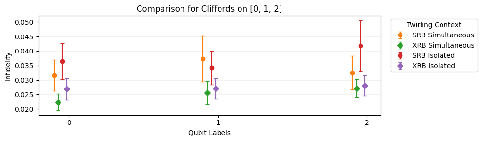
Compares SRB and XRB infidelities vs twirling groups.

Note

This class typically should not be invoked directly by users; the main plotting method is exposed dynamically by the attributes trueq.CircuitCollection.plot and trueq.estimate.EstimateCollection.plot if relevant.

static plot(fit, axes=None, filename=None)

Plots a comparison of process infidelity e_F measured by SRB and/or stochastic fidelity e_S measured by XRB. The comparison is made across twirling groups and is the natural plotting function for make_crosstalk_diagnostics().

import trueq as tq

circuits = tq.make_crosstalk_diagnostics([0, 1, 2], [4, 32])
tq.Simulator().add_depolarizing(0.05).run(circuits)
circuits.plot.compare_rb()

Parameters:

fit (EstimateCollection | CircuitCollection) – A collection of circuits or their fit.
axes (Iterable) – An iterable of existing axes. If none are provided, new axes are created. Note that axis instances can be repeated in this list if you want to force the combination of subfigures that would normally be distinct, see axes() for an example.
filename (str) – An optional filename to save the file as. The extension determines the filetype; common choices are “.png”, “.pdf”, and “.svg”. If no extension is given, PNG is chosen.

Compare Twirl

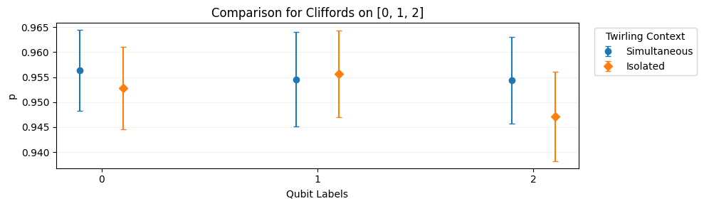
class trueq.visualization.plotters.comparisons.compare_twirl

Very generic plotter that compares like estimates across subsystems of a multi-system register.

Note

This class typically should not be invoked directly by users; the main plotting method is exposed dynamically by the attributes trueq.CircuitCollection.plot and trueq.estimate.EstimateCollection.plot if relevant.

static plot(fit, names, axes=None, filename=None)

Plots a comparison of the value of one or more estimates specified by names. The comparison is made across twirling groups. For example, if some protocol like SRB is performed on qubits in isolation as well as simultaneously, then this function can be used to compare these situations for any of the reported estimates.

import trueq as tq

circuits = tq.make_crosstalk_diagnostics([0, 1, 2], [4, 32])
tq.Simulator().add_depolarizing(0.05).run(circuits)
circuits.plot.compare_twirl("p")

Parameters:

fit (EstimateCollection | CircuitCollection) – A collection of circuits or their fit.
names (Iterable | str) – A name or list of names specifying which estimate parameters should be included in the plot.
axes (Iterable) – An iterable of existing axes. If none are provided, new axes are created. Note that axis instances can be repeated in this list if you want to force the combination of subfigures that would normally be distinct, see axes() for an example.
filename (str) – An optional filename to save the file as. The extension determines the filetype; common choices are “.png”, “.pdf”, and “.svg”. If no extension is given, PNG is chosen.

IRB Summary

class trueq.visualization.plotters.irb.irb_summary

Plots estimate fits from IRB.

Note

This class typically should not be invoked directly by users; the main plotting method is exposed dynamically by the attributes trueq.CircuitCollection.plot and trueq.estimate.EstimateCollection.plot if relevant.

static plot(fit, axes=None, filename=None)

Plots data from an IRB experiment. Relevant information from associated SRB and XRB experiments is also shown, see the IRB guide for details.

Parameters:

fit (EstimateCollection | CircuitCollection) – A collection of circuits or their fit.
axes (Iterable) – An iterable of existing axes. If none are provided, new axes are created. Note that axis instances can be repeated in this list if you want to force the combination of subfigures that would normally be distinct, see axes() for an example.
filename (str) – An optional filename to save the file as. The extension determines the filetype; common choices are “.png”, “.pdf”, and “.svg”. If no extension is given, PNG is chosen.

NOX

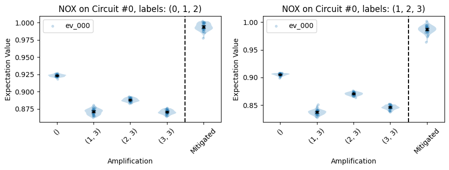
class trueq.visualization.plotters.mitigation.raw_nox

Plots the estimates of the individual NOX circuits alongside the mitigated estimates.

Note

This class typically should not be invoked directly by users; the main plotting method is exposed dynamically by the attributes trueq.CircuitCollection.plot and trueq.estimate.EstimateCollection.plot if relevant.

static plot(fit, observables=None, amplifications=None, show_imaginary=True, n_columns=3, axes=None, filename=None, legend=True)

Plots a summary of the NOX data for each applicable estimate, displaying subplots that show diagnostic information of the individual NOX circuits.

These plots can quickly tell you, e.g., if the number of NOX circuits is too small to guarantee the desired levels of statistical accuracy.

import trueq as tq
from trueq.simulation import GateMatch

# a simple circuit
circuit = tq.Circuit()
circuit += {(0, 1): tq.Gate.cx, (2, 3): tq.Gate.cx}
circuit += {(1, 2): tq.Gate.cx}
circuit += {(0, 1): tq.Gate.cx, (2, 3): tq.Gate.cx}
circuit.measure_all()

# generate the nox circuits
circuits = tq.make_nox(circuit)

# instantiate a simulator
sim = tq.Simulator().add_depolarizing(0.02, match=GateMatch(tq.Gate.cx))
sim.run(circuits, n_shots=10000)

# fit the data
labels = ((0, 1, 2), (1, 2, 3))
observables = ["000", "111"]
fit = circuits.fit(labels=labels, observables=observables)

# plot the estimates
fit.plot.raw_nox(observables=["000"])

Parameters:

fit (EstimateCollection | CircuitCollection) – A collection of circuits or their fit.
observables (list | NoneType) – A list of strings representing observables specifying which expectation values to plot, e.g. '000', 'ZIZ' or 'W01W02W00'. If observables == None, the plotter shows the expectation value of every observable in fit. Otherwise, the plotter shows the expectation value of every observable in observables that is also in fit. Default is None.
amplifications (list) – A list of tuples (marker, rep), where marker is the marker of a cycle being replaced by identity insertion and rep is the number of cycles that replace it. If amplifications == None, the plotter shows the expectation values of every NOX circuit, as well as the mitigated estimates. Otherwise, it shows the expectation values of each NOX circuit whose key.amplification is contained in amplifications, alongside the mitigated expecation values. Default is None.
show_imaginary (bool) – Whether to plot the imaginary components of complex expectation values. Default is True.
n_columns (int) – If new axes are made, how many columns in the grid to use.
axes (Iterable) – An iterable of existing axes. If none are provided, new axes are created. Note that axis instances can be repeated in this list if you want to force the combination of subfigures that would normally be distinct, see axes() for an example.
filename (str) – An optional filename to save the file as. The extension determines the filetype; common choices are “.png”, “.pdf”, and “.svg”. If no extension is given, PNG is chosen.
legend (bool) – Whether or not the legend should be plotted. Default is True.

KNR Heatmap

class trueq.visualization.plotters.nr.knr_heatmap

Plots KNR data as a heatmap.

Note

This class typically should not be invoked directly by users; the main plotting method is exposed dynamically by the attributes trueq.CircuitCollection.plot and trueq.estimate.EstimateCollection.plot if relevant.

static plot(fit_or_circuits, graph=None, width=None, cutoff=0.2, cutoff_relative_to_max=True, cutoff_ci=0.95, common_ylim=True, single_colorbar=True)

Plots all KNR data given in a single figure divided by whitespace into rows and columns of subplots. Each column of subplots corresponds to a unique cycle that was diagnosed with KNR, and each row of subplots corresponds to a different weight of error modes. Y-axis labels indicate which error occurred, and x-axis labels indicate which part of the cycle the error occurred on.

All reported errors are marginal errors. For example, if for a cycle {0: tq.Gate.id, 1: tq.Gate.id, (2,3): tq.Gate.cnot} it is reported that \(Z\) error occurs on 1: I with probability 0.1, then this is the sum of the probabilities of all length-4 Pauli errors with a \(Z\) on qubit 1. This particular error could in fact be part of a \(Z\otimes Z\) error on qubits 0 and 1 in the context of this cycle; you should look for this term in the heatmap to check.

Some Pauli errors cannot be distinguished from each other using the KNR protocol depending on the symmetries of a particular gate. Such indistinguishable errors are grouped together with commas in the y-labels. For example, \(IZ\) cannot be distinguished from \(ZZ\) in a CNOT gate.

Parameters:

fit_or_circuits (CircuitCollection | EstimateCollection) – A circuit collection with KNR data, or an estimate collection with KNR fits.
graph (Graph) – A Graph object to display device topologies at the top of columns.
width (float | NoneType) – The width of the figure in inches, or None for automatic.
cutoff (float) – A value below which data will not be displayed; a row of the plot will be hidden if every probability in the row is below the cutoff. This cutoff may be given in relative or absolute units, see cutoff_relative_to_max.
cutoff_relative_to_max (bool) – Whether cutoff is a fraction of the maximum error probability in the entire dataset, or whether it is absolute.
cutoff_ci (float) – A value of 0.95 here indicates that a probability value is considered below cutoff if its estimator is below the cutoff with 95% confidence.
common_ylim (float | bool) – A common maximum value for every color scale, or True to pick the maximum over all subplots, or False to have a different color scale for every subplot row.
single_colorbar (bool) – If common_ylim is not False, whether to draw a single color bar, or one identical colorbar for each subplot.

Raw

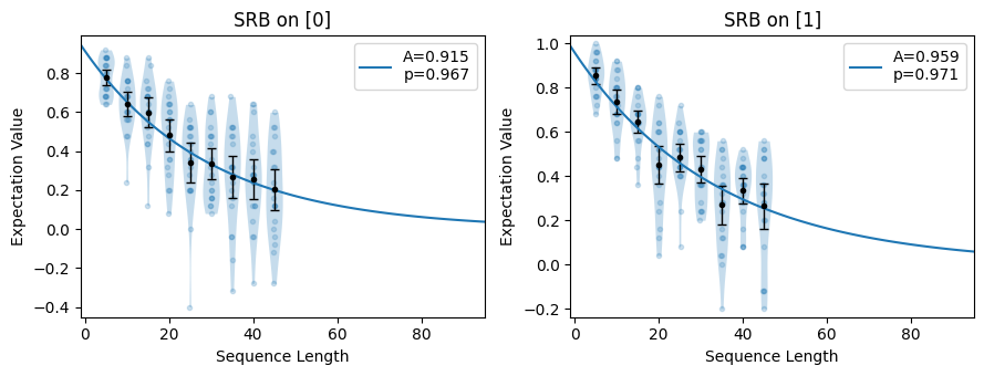
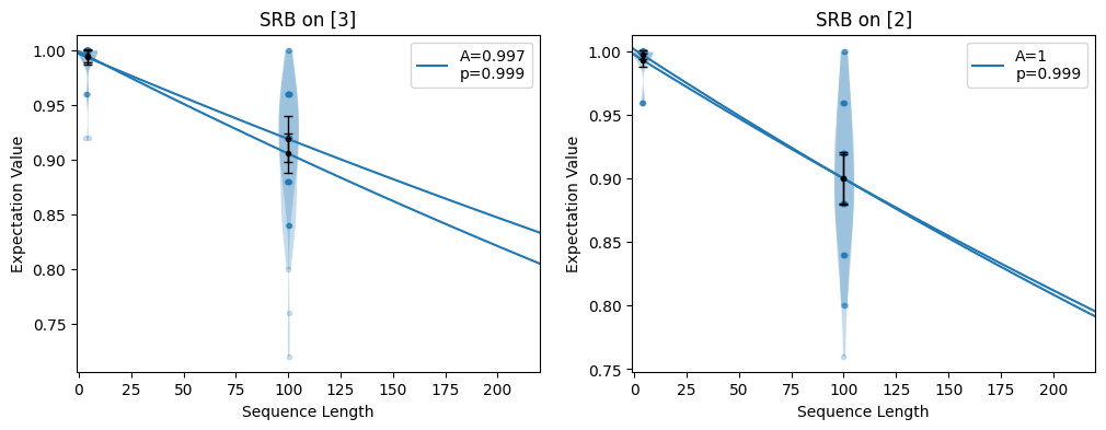
class trueq.visualization.plotters.raw.raw

Very generic plotter that overlays exponential fits onto lightly processed data.

Note

This class typically should not be invoked directly by users; the main plotting method is exposed dynamically by the attributes trueq.CircuitCollection.plot and trueq.estimate.EstimateCollection.plot if relevant.

static plot(fit, labels=None, show_imaginary=True, n_columns=3, axes=None, filename=None, legend=True)

Plots a summary of raw data for each applicable circuit collection. Also fits all applicable data to exponential curves and displays this too.

These plots are diagnostic tools which can quickly tell you if your sequence lengths are way off, or if there has been some systematic error in data entry or circuit conversion to your format.

import trueq as tq

circuits = tq.make_srb([0, 1], range(5, 50, 5), 20)
tq.Simulator().add_overrotation(0.08).add_depolarizing(0.02).run(circuits)

# show the exponential decays
circuits.plot.raw()

Parameters:

fit (EstimateCollection | CircuitCollection) – A collection of circuits or their fit.
labels (Iterable) – A list of labels (or list of lists of labels) specifying which qubit subset (or list of qubit subsets) to marginalize over.
show_imaginary (bool) – Whether to plot the imaginary components of complex decays.
n_columns (int) – If new axes are made, how many columns in the grid to use.
axes (Iterable) – An iterable of existing axes. If none are provided, new axes are created. Note that axis instances can be repeated in this list if you want to force the combination of subfigures that would normally be distinct, see axes() for an example.
filename (str) – An optional filename to save the file as. The extension determines the filetype; common choices are “.png”, “.pdf”, and “.svg”. If no extension is given, PNG is chosen.
legend (bool) – Whether or not the legend should be plotted. Default is True.

PlottingSuite

class trueq.visualization.plotters.PlottingSuite(parent=None)

A collection of Plotters, which are accessible as methods of instances of this class. Which plotters are present in the namespace is dependent on the parent object passed in at initialization. For example, a plotting function to do with XRB will only be present if the given parent has data for XRB.

Parameters:: parent (EstimateCollection | CircuitCollection) – A circuit collection or estimate collection to store plotters for.

Plotter

class trueq.visualization.plotters.abstract.Plotter

Represents a function that performs a plotting operation either on a EstimateCollection or a CircuitCollection (with data).

abstract static applies_to_estimates(keys)

A fast check that determines whether these estimates are broadly compatible with this plotting function. The plotting function is still allowed to raise (and indeed, it is encouraged) if it sees something it doesn’t like; this method is an a priori check that determines which plotters are automatically recommended to users.

Parameters:: keys (KeySet) – Keys of the EstimateCollection.
Return type:: bool

abstract static applies_to_circuits(keys)

A fast check that determines whether these circuits are broadly compatible with this plotting function. The plotting function is still allowed to raise (and indeed, it is encouraged) if it sees something it doesn’t like; this method is an a priori check that determines which plotters are automatically recommended to users.

This method should usually check to see if at least some data is present.

Parameters:: keys (KeySet) – Keys of the EstimateCollection.
Return type:: bool

abstract static plot(): Plots the given EstimateCollection or CircuitCollection.

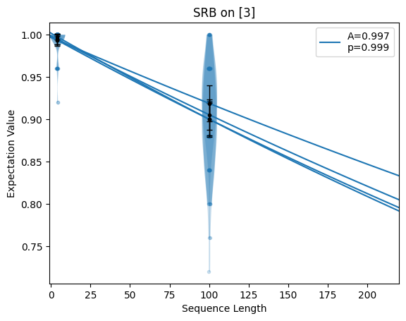
static axes(n_plots, axes=None, n_columns=1, axis_size=(4, 3.5), gs_options=None)

Returns an iterable of at least n_plots matplotlib axes. If axes are given, those axes are returned (and repeated if there are not enough of them). If no axes are given, new axes on a grid are created using given estimates.

import trueq as tq
import matplotlib.pyplot as plt

circuits = tq.make_srb([0, 1, 2, 3], [4, 100])
tq.Simulator().add_depolarizing(0.001).run(circuits)

# plot all decays on one axis
fig = plt.figure()
circuits.plot.raw(axes=plt.gca())

# plot all decays on two axes in a particular order
fig = plt.figure(figsize=(12, 4))
ax1, ax2 = plt.subplot(1, 2, 1), plt.subplot(1, 2, 2)
circuits.plot.raw(axes=[ax1, ax2, ax2, ax1])

Parameters:

n_plots (int) – How many subfigures there will nominally be.
axes (Iterable) – An iterable of existing axes. If none are provided, new axes are created. Note that axis instances can be repeated in this list if you want to force the combination of subfigures that would normally be distinct.
n_columns (int) – If new axes are made, how many columns in the grid to use.
axis_size (tuple) – A shape tuple to use to determine the size of each subfigure.
gs_options (dict) – Options to pass to matplotlib.gridspec.GridSpec.

Returns:

A tuple (axiter, finalize) where axiter is an iterator over axes, and finalize is a method to be called before the plotting function returns (this does file saving and layout tightening).

Return type:

tuple

static savefig(filename, fig=None)

Saves the given or current figure to disk as the given filename. Saves as a PNG if no filename is given.

Parameters:

filename (str) – The filename to save as.
fig (matplotlib.Figure | NoneType) – A matplotlib figure to save, or None to use the current figure.

Timestamps

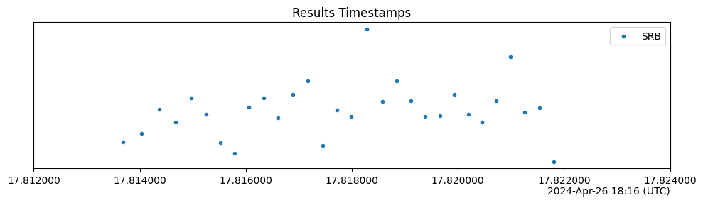
class trueq.visualization.plotters.timestamps.timestamps

Plots the timestamps of circuit results.

Note

This class typically should not be invoked directly by users; the main plotting method is exposed dynamically by the attributes trueq.CircuitCollection.plot and trueq.estimate.EstimateCollection.plot if relevant.

static plot(circuits, timezone=None, axis=None, filename=None, **filter)

Plots the timestamp of each result in the given circuit collection, sorted by protocol type. These timestamps are taken from the Results.last_modified attribute of each circuit with existing results—it is assumed that these values are parsable by dateutil.parser.parse.

The y-axis is meaningless; values are chosen randomly to distinguish circuits with nearly equal timestamps.

import trueq as tq

# make 30 circuits
circuits = tq.make_srb(0, 5, 30)

# this simulator updates the results attribute of each circuit in turn, and
# new Results objects get timestamps on instantiation
tq.Simulator().run(circuits)

circuits.plot.timestamps()

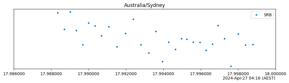
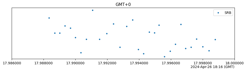
The timezone displayed on the x-axis is set to your local timezone by default, but can be changed to any timezone by providing the timezone argument. The displayed timezone is completely independent of any timezone information present in the result timestamps—the relevant conversions takes place automatically. If these timestamps do not contain any timezone information, then it is assumed that they represent UTC times.

import trueq as tq

# make 30 circuits and populate their results
circuits = tq.make_srb(0, 5, 30)
tq.Simulator().run(circuits)

circuits.plot.timestamps(timezone="Australia/Sydney")

# The pytz package is a bit more comprehensive and not OS-dependent
# You can get timezones from there, too.
import pytz

# list of all timezones
print(pytz.all_timezones[:5] + ["..."])
circuits.plot.timestamps(timezone=pytz.timezone("GMT+0"))

['Africa/Abidjan', 'Africa/Accra', 'Africa/Addis_Ababa', 'Africa/Algiers', 'Africa/Asmara', '...']

Parameters:

circuits (CircuitCollection) – A circuit collection.
timezone (str | datetime.tzinfo) – The timezone to use on the x-axis.
axis (matplotlib.Axis) – An existing axis to plot on.
filename (str) – An optional filename to save the file as. The extension determines the filetype; common choices are “.png”, “.pdf”, and “.svg”. If no extension is given, PNG is chosen.
**filter – A filter to apply to the datastructure, for example, circuits.plot.timestamps(protocol="SRB").