Download
Download this file as Jupyter notebook: knr_emulator.ipynb.
Example: Emulating a device from measured error profiles
In this example, we will see how to use the data from error diagnostics routines to construct a realistic emulator of a quantum processor.
For the sake of this example, the device in question will also be a simulator.
To avoid confusion, we will name it device. Our device will be a
minimalistic 3-qubit processor vulnerable to 2 noise sources. The first source
consists of relaxation processes, and the second source consists of unitary
overrotations of the entangling operations. The overrotation percentages are
different for each of the two possible entanglers. This first code block deals
only with initializing the device simulator; if you are interested solely
in creating an emulator from KNR data retrieved from a device or simulator,
skip to this subsection.
[2]:
import matplotlib.pyplot as plt
import trueq as tq
import trueq.simulation as tqs

# initiate a simulator
device = tq.Simulator()

# define time scales for single- and two-qubit gates
t_single_qb_gate = 50e-9
# 50 ns single-qubit gates
t_entangling_gate = 450e-9
# 450 ns entangling gates

# define time scales for relaxation processes
t1 = 100e-6  # 100 us population relaxation time
t2 = 100e-6  # 100 us phase relaxation time

# add a relaxation noise source based on the time scales above
device.add_relaxation(
    t1=t1, t2=t2, t_single=t_single_qb_gate, t_multi=t_entangling_gate
)

# define matches for introducing entangling operations with different fidelities
entangler_01_match = tqs.LabelMatch((0, 1)) & tqs.GateMatch(tq.Gate.cx)
entangler_12_match = tqs.LabelMatch((1, 2)) & tqs.GateMatch(tq.Gate.cx)

# add different unitary overrotation noise sources depending on the entangler
device.add_overrotation(multi_sys=0.12, match=entangler_01_match)
device.add_overrotation(multi_sys=0.08, match=entangler_12_match)
[2]:
<trueq.simulation.simulator.Simulator at 0x7f7293206af0>
Acquiring error profiles
Now that our device is properly defined, let’s pretend that we don’t know the underlying error profile, and that we wish to learn it. To do so, let’s perform typical KNR experiments on two hard cycles, each defined respectively by a \({\rm CNOT}\) operation between qubit \(0\) (control) and \(1\) (target) and by a \({\rm CNOT}\) operation between qubit \(1\) (control) and \(2\) (target). Since the former has a significantly worse infidelity than the latter (as seen in the device simulator above), their respective KNR sequences necessitate slightly different numbers of random cycles to yield better estimates (see the Selecting Parameters for Error Diagnostics example).
[3]:
# define the twirl over all three qubits to ensure thorough diagnostics
twirl = tq.Twirl("P", (0, 1, 2))

# define the cycles of interest for the diagnostics
cycle1 = tq.Cycle({(0, 1): tq.Gate.cx})
cycle2 = tq.Cycle({(1, 2): tq.Gate.cx})

# initialize a circuit collection with KNR circuits to characterize each hard cycle
knr_circuits = tq.make_knr(
    cycle1, n_random_cycles=[4, 16, 24], n_circuits=30, subsystems=1, twirl=twirl
)
knr_circuits += tq.make_knr(
    cycle2, n_random_cycles=[4, 24, 32], n_circuits=30, subsystems=1, twirl=twirl
)

# run the circuits on our device
device.run(knr_circuits, n_shots=1e4)

# plot the error profile:
layout = tq.visualization.Graph.linear(3, show_labels=True)  # specify the chip layout
knr_circuits.plot.knr_heatmap(layout)  # plot the heatmap
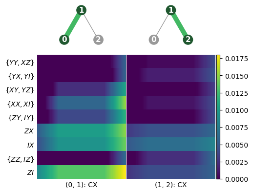
In the KNR heatmap above, we can see the reconstructed error profile
for each of the two hard cycles of interest. The labels on the left (e.g.
\(ZI\)) indicate specific errors, and the heatmap associates those errors
with a probability. The cycle whose noise profile is plotted on the left,
cycle1, is significantly noisier than cycle2, with some errors
reaching a probability of roughly \(1.2\%\). Note that the accuracy of
the emulator is limited by the quality of the error diagnostics. For
instance, in the above reconstructed map, some error probabilities have an
uncertainty associated to them, as observed by the varying color spectrum in
each of the heatmap’s cells. Moreover, certain errors are sometimes conflated
(e.g. \(\{IZ,ZZ\}\)), meaning that the diagnostic protocol couldn’t
distinguish which of the errors occured. In our case, the conflated errors
are not expected to be a problem because they occur with very low probability
compared to the dominant errors.
Using the reconstructed error profiles to make an emulator
Once the KNR circuits are run, an emulator can be easily constructed
by instantiating a new Simulator and adding the measured
error profile via the add_knr_noise() method:
[4]:
emulator = tq.Simulator().add_knr_noise(knr_circuits)
To see if our emulator correctly mimics the device, let’s submit a
circuit to each and compare the distribution of results. In this example, we
choose a circuit that ideally produces a GHZ state \(|\psi\rangle = (|
000\rangle+ | 111 \rangle)/\sqrt{2}\):
[5]:
cycle0 = tq.Cycle({0: tq.Gate.h})
circuit = tq.Circuit([cycle0, cycle1, cycle2])
circuit.measure_all()
circuit.draw()
[5]:
Note that the emulator is meant to mimic the device in the context
where Randomized Compiling is applied (see RC). Hence, let’s
generate RC circuits and sample results for both the device and the
emulator:
[6]:
# randomly compile the test circuit
rc_circuits = tq.randomly_compile(circuit, n_compilations=30)

# sample the randomly compiled versions of the circuit on the device
device_results = sum(
    device.sample(rc_circuit, n_shots=1e3) for rc_circuit in rc_circuits
)

# sample the randomly compiled versions of the circuit on the emulator
emulator_results = sum(
    emulator.sample(rc_circuit, n_shots=1e3) for rc_circuit in rc_circuits
)
Now, let’s compare the results in a log-scaled histogram to zoom in on the small faulty outcomes:
[7]:
tq.visualization.plot_results(
    device_results, emulator_results, labels=["Device", "Emulator"]
)

plt.gca().set_yscale("log")
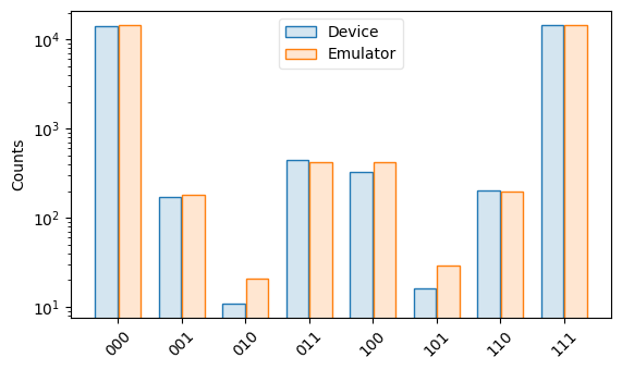
Notice that the emulator and the device yield very similar output
distributions. Of course, the two histograms differ slightly, and this can be
due to two causes. First, the results displayed in the histograms were
obtained from finite measurement samples, and are therefore susceptible to
small statistical deviations. Due to the logarithmic scaling of the plot,
these statistical deviations are visually amplified for unlikely outcomes such
as \(010\) and \(101\). Second, the emulator originates from
approximated error profiles. Small inaccuracies in the reconstructed error
profiles may in turn yield small inaccuracies in the emulator.
Download
Download this file as Jupyter notebook: knr_emulator.ipynb.