Download
Download this file as Jupyter notebook: xrb_example.ipynb.
Example: Running XRB
This example illustrates how to generate extended randomized benchmarking
(XRB) circuits and use them to estimate the probability of a stochastic
error acting on the specified system(s) during a random gate. While this example uses
the built-in Simulator to execute the circuits, the same
procedure can be followed for hardware applications.
Isolated XRB
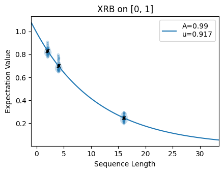
This section illustrates how to generate XRB circuits to characterize a pair of qubits in isolation. Here, we are performing two-qubit XRB which learns the stochastic infidelity over the two-qubit Clifford gateset.
[2]:
import trueq as tq

# generate XRB circuits to characterize a pair of qubits [0, 1]
# with 9 * 30 random circuits for each circuit depth [2, 4, 16]
circuits = tq.make_xrb([[0, 1]], [2, 4, 16], 30)

# initialize a noisy simulator with stochastic Pauli and overrotation
sim = tq.Simulator().add_stochastic_pauli(px=0.02).add_overrotation(0.04)

# run the circuits on the simulator to populate their results
sim.run(circuits, n_shots=1000)

# plot the exponential decay of the purities
circuits.plot.raw()
Print the fit summary:
[3]:
circuits.fit()
[3]:
|
XRB
Extended Randomized Benchmarking
|
Cliffords
(0, 1)
|
|
${e}_{S}$
The probability of a stochastic error acting on the specified systems during a random gate.
|
4.0e-02 (7.7e-04)
0.03964839003461862, 0.0007715144117231922
|
|
${u}$
The unitarity of the noise, that is, the average decrease in the purity of an initial state.
|
9.2e-01 (1.6e-03)
0.9170935624139733, 0.0015806402291410383
|
|
${A}$
SPAM parameter of the exponential decay $Au^m$.
|
9.9e-01 (9.0e-03)
0.9901245371245811, 0.009009681915540932
|
Simultaneous XRB
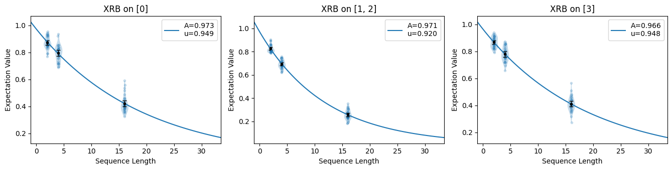
This section demonstrates how to generate XRB circuits that characterize the amount of stochastic noise while gates are applied simultaneously on a device.
For example, to generate XRB circuits to simultaneously characterize a single qubit
[0], a pair of qubits [1, 2], and another single qubit [3] with
\(9 \times 30\) random circuits for each circuit depth [2, 4, 16], we can
write:
[4]:
circuits = tq.make_xrb([[0], [1, 2], [3]], [2, 4, 16], 30)

# initialize a noisy simulator with stochastic Pauli and overrotation
sim = tq.Simulator().add_stochastic_pauli(px=0.02).add_overrotation(0.04)

# run the circuits on the simulator to populate their results
sim.run(circuits, n_shots=1000)

# plot the exponential decay of the purities
circuits.plot.raw()
Print the fit summary:
[5]:
circuits.fit()
[5]:
|
XRB
Extended Randomized Benchmarking
|
Cliffords
(0,)
|
Cliffords
(1, 2)
|
Cliffords
(3,)
|
|
${e}_{S}$
The probability of a stochastic error acting on the specified systems during a random gate.
|
1.9e-02 (7.8e-04)
0.019252635636475723, 0.0007790272643924942
|
3.8e-02 (1.0e-03)
0.038128274294094266, 0.0010368039759344782
|
2.0e-02 (7.2e-04)
0.019701537381388357, 0.0007232024276490294
|
|
${u}$
The unitarity of the noise, that is, the average decrease in the purity of an initial state.
|
9.5e-01 (2.0e-03)
0.9491538569413327, 0.0020374104968540405
|
9.2e-01 (2.1e-03)
0.9202103644932877, 0.002127514516375127
|
9.5e-01 (1.9e-03)
0.9479801010832181, 0.00189054460796371
|
|
${A}$
SPAM parameter of the exponential decay $Au^m$.
|
9.7e-01 (1.1e-02)
0.9730845881357387, 0.011412005184361088
|
9.7e-01 (9.5e-03)
0.9706836022041112, 0.009483239490881932
|
9.7e-01 (1.0e-02)
0.9658482484676595, 0.01012431702498326
|
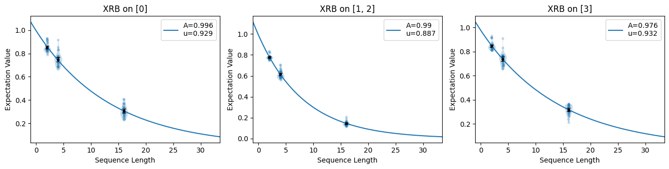
Simultaneous XRB on Qudits
The make_xrb() function can be used for qudits of higher dimension in
exactly the same way as for qubits. For example, consider the same simultaneous
characterization configuration as in the example above but with qutrits instead of
qubits:
[6]:
# set the global dimension to 3 for qutrits
tq.settings.set_dim(3)

# create circuits for the simultaneous characterization of
# qutrit 1, the qutrit pair (1, 2) and qutrit 3:
circuits = tq.make_xrb([[0], [1, 2], [3]], [2, 4, 16], 30)

# display a sample circuit
circuits[0].draw()
[6]:
We again initialize a noisy simulator with overrotation errors and stochastic Pauli
noise. The add_overrotation() method works natively for
qudits of higher dimension. To implement the stochastic noise, we use a probabilistic
sum of Weyl operators, analogous to the stochastic Pauli channel used for qubits. We
add this noise to our simulator using the
add_stochastic_weyl() method. For this example, we add a
small qutrit \(X\) and \(X^2\) error:
[7]:
sim = tq.Simulator().add_stochastic_pauli(W10=0.02, W20=0.01).add_overrotation(0.04)

# run the circuits on the simulator to populate their results
sim.run(circuits, n_shots=1000)

# plot the exponential decay of the purities
circuits.plot.raw()
Display the fit parameter:
[8]:
circuits.fit()
[8]:
|
XRB
Extended Randomized Benchmarking
|
Cliffords
(0,)
|
Cliffords
(1, 2)
|
Cliffords
(3,)
|
|
${e}_{S}$
The probability of a stochastic error acting on the specified systems during a random gate.
|
3.2e-02 (9.6e-04)
0.03208522872567443, 0.0009587915032335817
|
5.7e-02 (9.0e-04)
0.05730118855628075, 0.0009025833049068695
|
3.1e-02 (7.6e-04)
0.030563616891930545, 0.000762786516217963
|
|
${u}$
The unitarity of the noise, that is, the average decrease in the purity of an initial state.
|
9.3e-01 (2.1e-03)
0.9289663800074087, 0.002088064031742223
|
8.9e-01 (1.7e-03)
0.8872895622111183, 0.0017230000227484161
|
9.3e-01 (1.7e-03)
0.9322827635053625, 0.0016638142530733804
|
|
${A}$
SPAM parameter of the exponential decay $Au^m$.
|
1.0e+00 (1.1e-02)
0.9957762645484559, 0.011187114159611102
|
9.9e-01 (8.7e-03)
0.9899700211346119, 0.008712167211532047
|
9.8e-01 (9.6e-03)
0.9762061135717386, 0.009575470438259721
|
Download
Download this file as Jupyter notebook: xrb_example.ipynb.