---

Download

Download this file as Jupyter notebook: intro.ipynb.

Example: Introduction to the Simulator

True-Q™ offers a highly versatile Simulator that allows users to simulate arbitrary circuits with a wide variety of noise models and options for noise model customization. In particular, the simulator can be used to:

1. Simulate the final quantum state of a circuit. This will be a pure state vector if the noise model is ideal or has only unitary noise, and will be a density matrix otherwise.

2. Simulate the total effective operator of a circuit. This will be a unitary matrix if the noise model is ideal or has only unitary noise, and will be a superoperator otherwise.

3. Sample a given number of bitstrings (or ditstrings if higher energy levels are defined) from the distribution defined by the final simulated quantum state of a circuit. These results can be returned, or can be automatically populated into the respective results attributes of the given circuits.

In this example, we go through the basic features of the True-Q™ simulator. We begin by instantiating a circuit to play with:

import numpy as np
import trueq as tq


circuit = tq.Circuit([{0: tq.Gate.x, 1: tq.Gate.y}, {(0, 1): tq.Gate.cz}])
circuit.measure_all()
circuit.draw()

Simulator Basics

In its simplest configuration, a (noiseless) simulator can be instantiated from True-Q™’s Simulator class as follows:

sim = tq.Simulator()

We can use it to simulate the final state of the circuit, with all initial states prepared as \(|0\rangle\) by default. Since the simulator is noiseless, the output state is a pure state; a noisy simulator will generally return a density matrix instead.

sim.state(circuit).mat()

array([0.+0.j, 0.+0.j, 0.+0.j, 0.-1.j])

If we want to force the output to be a density matrix, we can use:

sim.state(circuit).upgrade().mat()

array([[0.+0.j, 0.+0.j, 0.+0.j, 0.+0.j],
       [0.+0.j, 0.+0.j, 0.+0.j, 0.+0.j],
       [0.+0.j, 0.+0.j, 0.+0.j, 0.+0.j],
       [0.-0.j, 0.-0.j, 0.-0.j, 1.+0.j]])

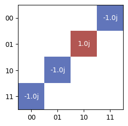
We can also use it to compute the overall action of the circuit. Since the simulator is currently noiseless, the output is a unitary matrix; a noisy simulator will return a superoperator (in the rowstacked basis).

tq.plot_mat(sim.operator(circuit).mat())

Finally, we can use a simulator to populate the results attribute of the circuit. Currently, this attribute is just an empty dictionary:

circuit.results

Results({}, dim=None)

But after calling the run() method, it has results that are randomly sampled bitstrings from the final state of a state simulation:

sim.run(circuit, n_shots=100)
circuit.results

Results({'11': 100})

In this case, all 100 shots end in the 11 state because the final state is a computational eigenstate.

When re-running the simulation, it will overwrite the existing results unless otherwise specified. Another option is to call the simulator’s sample() method which returns a Results object directly without affecting the circuit’s results attribute:

results = sim.sample(circuit, n_shots=100)
results

Results({'11': 100})

We can also specify infinite shots to get the expectation values of each bitstring:

sim.run(circuit, n_shots=np.inf, overwrite=True)
circuit.results

Results({'11': 1.0})

Adding Noise Sources

We construct a noisy simulator by appending noise sources to a noiseless simulator. The example below demonstrates this using two of True-Q™'s built-in noise sources:

# Add an overrotation noise, which causes single qubit gates to be simulated as U^1.02
sim.add_overrotation(single_sys=0.02)

# Add a depolarizing noise source at a rate of 0.8% per acted-on qubit per cycle
sim.add_depolarizing(p=0.008)

# Note that noisy simulators can be constructed as one-liners
other_sim = tq.Simulator().add_overrotation(single_sys=0.02).add_depolarizing(p=0.008)

Note

Note that simulation is cycle-based. Each noise source is called to add noise to the quantum state (or to the superoperator if operator() is called) for each cycle in a circuit. The order in which noise sources are applied is dictated by the order in which they were added to the simulator.

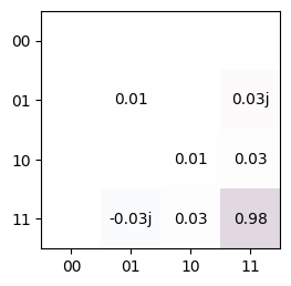
Now, since the simulator applies a depolarizing noise source, we get a density operator rather than a pure state:

tq.plot_mat(sim.state(circuit).mat())

After calling the run() method (overwriting the results from above), we end up with noisy outcomes:

sim.run(circuit, n_shots=100, overwrite=True)
circuit.results

Results({'11': 100})

For more information on both built-in and custom noise sources, check out Example: Advanced Simulator Usage next.

---

Download

Download this file as Jupyter notebook: intro.ipynb.