Download
Download this file as Jupyter notebook: irb_example.ipynb.
Example: Running IRB
This example page demonstrates how to use make_irb() method to
estimate the infidelity of a specific gate. This protocol differs from
Cycle Benchmarking (CB) in several ways:
It estimates the infidelity of a specific gate (not cycle) composed with gates from the twirling group, see Interleaved Randomized Benchmarking (IRB) for more details. Gate infidelity can then be estimated by taking into account the results of an SRB experiment.
IRB uses a different twirling group than CB, Cliffords instead of Paulis by default. Paulis being a reference group with no entangling operations and therefore usually higher fidelity, leading to less systematic uncertainty in estimates.
Typically uses fewer circuits than CB.
IRB only gives information about specific gates (possibly in the context of being simultaneously applied), and not about entire cycles like CB.
We begin by defining some cycles that contain the gates we want to characterize using IRB. Next we generate IRB circuits for these cycles. Note that we could perform simultaneous two qubit IRB with a cycle such as:
{(1, 2): tq.Gate.cz, (3, 4): tq.Gate.cz}
See make_irb() for more details.
[2]:
import trueq as tq

cycle1 = {1: tq.Gate.h}
cycle2 = {2: tq.Gate.h}
cycle12 = {(1, 2): tq.Gate.cz}

# Generate a circuit collection to run IRB on the above cycles with 30 random circuits
# for each circuit length in [4, 32, 64]:
n_random_cycles = [4, 32, 64]
circuits = tq.make_irb(cycle1, n_random_cycles)
circuits += tq.make_irb(cycle2, n_random_cycles)
circuits += tq.make_irb(cycle12, n_random_cycles)
len(circuits)
[2]:
270
We are interested in the gate fidelity of the individual gates in the cycles defined
above, e.g. \(CZ\) alone, so we also need a reference SRB experiment to translate
from the average fidelity of cycles dressed with gates in the twirling group to
fidelity of the undressed gates. Optionally, to tighten the bound on the infidelity
estimate, we also do an XRB experiment. The double nesting [[1, 2]] is necessary
to characterize the \(CZ\) gate because just [1, 2] refers to simultaneous
single-qubit gates.
[3]:
circuits += tq.make_srb([1], n_random_cycles)
circuits += tq.make_srb([2], n_random_cycles)
circuits += tq.make_srb([[1, 2]], n_random_cycles)
circuits += tq.make_xrb([1], n_random_cycles)
circuits += tq.make_xrb([2], n_random_cycles)
circuits += tq.make_xrb([[1, 2]], n_random_cycles)
Create a noisy simulator in lieu of a physical device and populate all circuits with results.
[4]:
sim = tq.Simulator().add_depolarizing(0.01).add_overrotation(0.04)
sim.run(circuits)
Print a summary of the results for the CZ gate:
[5]:
circuits.fit()
[5]:
|
SRB
Streamlined Randomized Benchmarking
|
Cliffords
(1,)
|
Cliffords
(2,)
|
Cliffords
(1, 2)
|
|
${e}_{F}$
The probability of an error acting on the targeted systems during a random gate.
|
8.8e-03 (7.1e-04)
0.00881774949177988, 0.0007135525897545267
|
1.0e-02 (9.9e-04)
0.010094637642109994, 0.0009925258424418014
|
1.6e-02 (1.2e-03)
0.01633249131920554, 0.0011817696810949604
|
|
${p}$
Decay parameter of the exponential decay $Ap^m$.
|
9.9e-01 (9.5e-04)
0.9882430006776268, 0.0009514034530060355
|
9.9e-01 (1.3e-03)
0.9865404831438533, 0.001323367789922402
|
9.8e-01 (1.3e-03)
0.9825786759261808, 0.0012605543265012912
|
|
${A}$
SPAM parameter of the exponential decay $Ap^m$.
|
9.5e-01 (2.2e-02)
0.9496943114342195, 0.022158649177850077
|
9.7e-01 (2.4e-02)
0.9682811612265126, 0.024220009958355576
|
1.0e+00 (2.3e-02)
1.0235410427144767, 0.022704625061970362
|
|
XRB
Extended Randomized Benchmarking
|
Cliffords
(1,)
|
Cliffords
(2,)
|
Cliffords
(1, 2)
|
|
${e}_{U}$
The process infidelity of the coherent error acting on the specifed systems during a random gate.
|
2.5e-03 (9.1e-04)
0.0025482653409639178, 0.0009130799903846304
|
4.5e-03 (1.1e-03)
0.004455486006029352, 0.001110310956031211
|
4.0e-03 (1.2e-03)
0.004037810987254628, 0.0012461380271334172
|
|
${e}_{S}$
The probability of a stochastic error acting on the specified systems during a random gate.
|
6.3e-03 (5.7e-04)
0.006269484150815963, 0.0005696997195851557
|
5.6e-03 (5.0e-04)
0.0056391516360806415, 0.0004976774770553055
|
1.2e-02 (4.0e-04)
0.012294680331950913, 0.0003953231633900052
|
|
${u}$
The unitarity of the noise, that is, the average decrease in the purity of an initial state.
|
9.8e-01 (1.5e-03)
0.9833337841731805, 0.0015096746565933126
|
9.9e-01 (1.3e-03)
0.9850046623453513, 0.0013196559954568763
|
9.7e-01 (8.3e-04)
0.9739325850672672, 0.0008329872884657269
|
|
${A}$
SPAM parameter of the exponential decay $Au^m$.
|
1.0e+00 (3.3e-02)
1.006206653809557, 0.03295414862137787
|
9.9e-01 (3.1e-02)
0.9857698015908191, 0.031034223527471427
|
1.0e+00 (1.9e-02)
1.0359914930836414, 0.019449275198710116
|
|
IRB
Interleaved Randomized Benchmarking
|
Cliffords
(1,) : Gate.h
|
Cliffords
(2,) : Gate.h
|
Cliffords
(1, 2) : Gate.cz
|
|
${e}_{F}$
The probability of an error acting on the targeted systems during a dressed gate of interest.
|
1.8e-02 (1.8e-03)
0.018386882900838702, 0.0018077301395741684
|
2.1e-02 (2.4e-03)
0.02074658647365038, 0.002427310264746314
|
3.5e-02 (5.0e-03)
0.03479625392956192, 0.0049757600310042
|
|
${e}_{IU}$
An upper bound on the inferred value of $e_F$ that accounts for systematic errors in the interleaved estimate.
|
2.6e-02 (4.4e-03)
0.02586904417929753, 0.00436243853059833
|
3.6e-02 (5.1e-03)
0.0360211894560529, 0.005143846364291683
|
4.6e-02 (8.4e-03)
0.045946712207948805, 0.00835926458832259
|
|
${e}_{IL}$
A lower bound on the inferred value of $e_F$ that accounts for systematic errors in the interleaved estimate.
|
3.6e-03 (1.4e-03)
0.003599679840758152, 0.0013600618938340368
|
3.2e-03 (1.4e-03)
0.003197877382540598, 0.0014210160853860843
|
7.6e-03 (3.4e-03)
0.007618282603816633, 0.0033666587807032987
|
|
${p}$
Decay parameter of the exponential decay $Ap^m$.
|
9.8e-01 (2.4e-03)
0.9754841561322151, 0.002410306852765558
|
9.7e-01 (3.2e-03)
0.9723378847017995, 0.003236413686328419
|
9.6e-01 (5.3e-03)
0.9628839958084673, 0.00530747736640448
|
|
${A}$
SPAM parameter of the exponential decay $Ap^m$.
|
9.5e-01 (4.0e-02)
0.9451646389604796, 0.03950903684857499
|
9.6e-01 (5.2e-02)
0.960563962171888, 0.05215361153989234
|
1.0e+00 (8.7e-02)
1.0396388468156559, 0.08709345791149323
|
Plot a summary of information:
[6]:
circuits.plot.irb_summary()
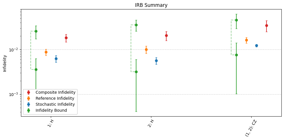
For a refresher on the parameters plotted above, see Interleaved Randomized Benchmarking (IRB).
Download
Download this file as Jupyter notebook: irb_example.ipynb.