---

Download

Download this file as Jupyter notebook: spam.ipynb.

Example: State Preparation and Measurement Noise

import trueq as tq
import numpy as np

Adding Measurement Bitflip Noise

The most convenient way to add measurement noise is through the add_readout_error() noise source. There are several ways to specify readout error with this method. Measurement noise is applied only when a simulator’s sample() or run() method is called.

The most basic method is to provide a single number. In the following example, each qubit will get a (symmetric) 1% bitflip error.

sim = tq.Simulator().add_readout_error(0.01)
circuit = tq.Circuit({range(5): tq.Meas()})
sim.run(circuit, n_shots=1000)
circuit.results

Results({'00000': 951, '00001': 11, '00010': 6, '00100': 12, '01000': 6, '10000': 14})

We can use a dictionary to specify the readout error of particular qubits. Qubits that are not explicitly assigned a readout error get no noise, or the specified default value. In this example, all qubits get 1% readout error, except qubit 1 gets a 50% readout error.

sim = tq.Simulator().add_readout_error(0.01, {1: 0.5})
circuit = tq.Circuit({range(5): tq.Meas()})
sim.run(circuit, n_shots=1000)
circuit.results

Results({'00000': 485, '00001': 7, '00010': 5, '10000': 7, '01000': 475, '01001': 4, '01010': 3, '01100': 7, '01110': 1, '11000': 6})

In both of the above examples, any probability can be replaced with a pair of probabilities [p10, p01], where p10 is the probability of flipping a ‘0’ to a ‘1’ right before measurement, and p01 is the probability of flipping a ‘1’ to a ‘0’ right before measurement. In the following example, qubits get 1% readout error, except qubit 1 gets 5% readout error, and qubit 3 get asymmetric readout error of 1% on \(|0\rangle\) and 7% on \(|1\rangle\).

sim = tq.Simulator().add_readout_error(0.01, {1: 0.05, 3: [0.01, 0.07]})
circuit = tq.Circuit({range(5): tq.Meas()})
sim.run(circuit, n_shots=1000)
circuit.results

Results({'00000': 918, '00001': 8, '00100': 16, '10000': 10, '00010': 6, '01000': 42})

Specifying Confusion Matrices

We can also use the full confusion matrix anywhere in the add_readout_error() noise source. There isn’t any value to this for a single qubit confusion matrix because it is fully specified by a length-2 vector as described above, but if we are interested in adding misclassification into a third level, or correlated readout error, then a confusion matrix gives us control over all the probabilities. In the following example, we specify that 0 and 1 are misclassified as 2 with a small probability.

sim = tq.Simulator().add_readout_error([[0.98, 0.06], [0.01, 0.9], [0.01, 0.04]])
circuit = tq.Circuit({range(5): tq.Meas()})
sim.run(circuit, n_shots=1000)
circuit.results

Results({'00000': 909, '00001': 7, '00002': 4, '00010': 8, '00020': 7, '00100': 10, '00102': 1, '00200': 9, '01000': 8, '01020': 1, '02000': 9, '10000': 9, '10010': 1, '20000': 14, '20002': 1, '20010': 2}, dim=3)

Similarly, in the following example, we specify a correlated readout error on qubits 2 and 3, where the rows and columns are in the usual 00, 01, 10, 11 order.

confusion_mat = [
    [0.99, 0.05, 0.00, 0.00],
    [0.00, 0.90, 0.00, 0.02],
    [0.00, 0.05, 0.96, 0.00],
    [0.01, 0.00, 0.04, 0.98],
]
sim = tq.Simulator().add_readout_error(0, {(2, 3): confusion_mat})
circuit = tq.Circuit({range(5): tq.Meas()})
sim.run(circuit, n_shots=10000)
circuit.results

Results({'00000': 9914, '00110': 86})

Adding Measurement POVM Noise

Finally, as a more advanced option, measurement error can also be specified as a positive-operator valued measurement (POVM).

As a quick reminder (look elsewhere for a full description, e.g. Wikipedia or the lecture notes of John Watrous), a POVM is a set of positive-semi-definite matrices \(\{P_i\}_{i=1}^N\) that sum to the identity matrix, \(\sum_{i=1}^N P_i = \mathbb{I}\). The probability of observing the outcome \(i\) when measuring a state \(\rho\) is equal to \(p_i:=\operatorname{Tr}(\rho P_i)\). One can also take a POVM defined on a single qubit, and tensor it together to get a POVM on a collection of qubits. For example, if the POVM above describes measurement on a single qubit, the probability of measuring the outcomes \((i_0, i_1, i_2)\) on three qubits is simply \(p_{i_0}p_{i_1}p_{i_2}\). This is why we use the Tensor object as a primitive for specifying POVMs; its purpose is to store tensor project structures sparsely without actually taking kronecker products between subsystems unless necessary.

The add_readout_error() supports POVMs in addition to all the formats described in the previous section. A POVM is specified a 3D array where the first index \(i\) ranges over POVM elements \(P_i\).

In this example, we construct a coherent measurement error on qubit 3.

# Define a set of ideal POVM operators for each subsystem
proj0 = np.array([[1, 0], [0, 0]])  # project onto this one to get a "0"
proj1 = np.array([[0, 0], [0, 1]])  # project onto this one to get a "1"
ideal = np.array([proj0, proj1])

# Define a unitary rotation about X by 20 degrees
u = tq.Gate.from_generators("X", 20).mat

# Define noisy POVM operators by rotating the ideal POVM operators by U, which
# coherently changes the basis of the measurement
twisted_povm = [u @ x @ u.conj().T for x in ideal]

# initialize a simulator with the above POVM applied to qubit 3
sim = tq.Simulator().add_readout_error(0, {3: twisted_povm})
circuit = tq.Circuit({range(5): tq.Meas()})
sim.run(circuit, n_shots=1000)
circuit.results

Results({'00000': 980, '00010': 20})

In this example, we add a third measurement label even though the simulation is on qubits, so that the outcomes ‘0’, ‘1’, and ‘2’ are all possible.

Here we specify that the state \(|0\rangle\) results in the outcome ‘0’ 99% of the time, but also results in the outcome ‘2’ 1% of the time. Similarly, the state \(|1\rangle>`\) results in the outcome ‘1’ 70% of the time, but also results in ‘2’ 25% of the time and ‘0’ 5% of the time. This particular example could be more efficiently implemented as a confusion matrix, but is presented as a POVM for demonstration.

povm = [np.diag([0.99, 0.05]), np.diag([0, 0.7]), np.diag([0.01, 0.25])]
sim = tq.Simulator().add_readout_error(povm)
circuit = tq.Circuit([{1: tq.Gate.h}, {(0, 1): tq.Meas()}])
sim.run(circuit, n_shots=10000)
circuit.results

Results({'00': 5159, '20': 55, '01': 3434, '21': 47, '02': 1287, '22': 18}, dim=3)

Adding State Preparation Noise

State preparation noise can be added using the add_prep() noise source.

Note

The add_prep() noise source only takes place when a Prep() object is encountered. Many circuits do not have any Prep() objects unless explicitly added.

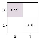
We can either enter the noise as the probability of a bitflip during preparation of \(|0\rangle\):

sim = tq.Simulator().add_prep(0.01)
circuit = tq.Circuit([{0: tq.Prep()}])
tq.plot_mat(sim.state(circuit).mat())

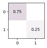
Or we can specify the pure state or density matrix we want to prepare with. Here a density matrix is used:

sim = tq.Simulator().add_prep([[0.75, 0], [0, 0.25]])
circuit = tq.Circuit([{0: tq.Prep()}])
tq.plot_mat(sim.state(circuit).mat())

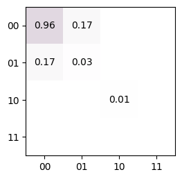
We can place different preparations on different qubits. Here, we have a 1% preparation bitflip error by default, but a 20 degree rotation error on qubit 3.

u = tq.Gate.from_generators("Y", 20).mat
sim = tq.Simulator().add_prep(0.01, {3: u @ np.diag([1, 0]) @ u.conj().T})
circuit = tq.Circuit([{0: tq.Prep(), 3: tq.Prep()}])
tq.plot_mat(sim.state(circuit).mat())

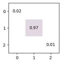
We can specify preparation states of larger dimension to add leakage levels.

sim = tq.Simulator().add_prep(np.diag([0.97, 0.02, 0.01]))
circuit = tq.Circuit([{0: tq.Prep()}, {0: tq.Gate.x}])
tq.plot_mat(sim.state(circuit).mat())

---

Download

Download this file as Jupyter notebook: spam.ipynb.