---

Download

Download this file as Jupyter notebook: sc_example.ipynb.

Example: Running Stochastic Calibration

This example will show how to characterize the noise acting on a system so that it can be corrected. We begin by initializing a noisy simulator with a 2-qubit rotation about $Z$ by some angle $\theta$. Then we show how to find $\theta$ using stochastic calibration.

import numpy as np
import trueq as tq

# make a noisy simulator
sim = tq.Simulator().add_depolarizing(p=0.001)
sim.add_overrotation(single_sys=0.01, multi_sys=0.01)

# adding a rotation by 12 degrees to the first qubit in every 2-qubit gate,
# i.e. Z(12) is the noise we are going to try to characterize
mat = tq.Gate.from_generators("Z", 12).mat
sim.add_kraus([np.kron(mat, np.eye(2))])

<trueq.simulation.simulator.Simulator at 0x7f0c48fddc10>

We are going to perform stochastic calibration for a $CZ$ gate. We choose to look at the $XI$ Pauli decay because it anticommutes with our suspected error, $ZI$. Equivalently, we could have chosen to use the $YI$ Pauli decay to characterize our $ZI$ error. To minimize the experimental footprint, we use data at a single sequence length as in [15].

cycle = tq.Cycle({(0, 1): tq.Gate.cz})

# generate SC circuits with 24 random cycles to get decays associated with XI
circuits = tq.make_sc(cycle, [24], pauli_decays=["XI"])
print(len(circuits))

30

Find the expectation value and standard deviation of the circuit when corrections of the form $Z(\varphi )$ are applied on the first qubit prior to each $CZ$ gate. The expectation values correspond to the $XI$ diagonal entry of the superoperator in the Pauli basis; values close to $1$ indicate that the suspected error is small.

# 20 equidistant points between -40 and 40 for trial values of phi
angles = np.linspace(-40, 40, 20)

all_circuits = tq.CircuitCollection()
for j, phi in enumerate(angles):
    # adds a Z(phi) rotation on qubit 0 gate before every CZ gate
    c = tq.compilation.CycleReplacement(
        cycle, replacement=[tq.Cycle({(0): tq.Gate.from_generators("Z", phi)}), cycle]
    )
    new_circs = tq.CircuitCollection(map(c.apply, circuits))

    # run circuit collection (with Z(phi)s inserted)
    sim.run(new_circs)

    # put all circuits into one callection, organized by the custom keyword "phi"
    all_circuits.append(new_circs.update_keys(phi=phi))

Plot the expectation values as a function of $\varphi$:

all_circuits.plot.compare("f_24_XI", "phi")

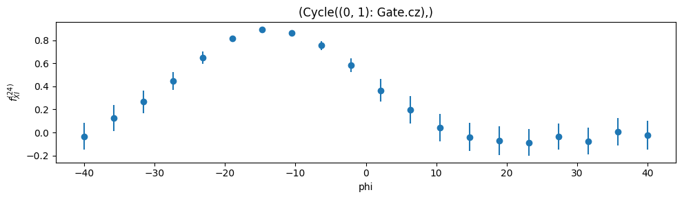
The y-axis is the expectation value after 24 (randomized) applications of the cycle of interest, and the x-axis is the correction angle we have compiled into the circuit. The maximum expectation value corresponds to the value of $XI$ closest to 1, so finding the angle at which the plot peaks tells us which angle to rotate by to correct the noise. The peak occurs at approximately $\varphi =-12$, which is consistent with the noise applied by the simulator.

---

Download

Download this file as Jupyter notebook: sc_example.ipynb.