Download
Download this file as Jupyter notebook: estimate_collections.ipynb.
Parsing Estimate Collections
The standard workflow for diagnostic and
suppression protocols is to invoke their
generation functions to create a circuit collection,
run each of the circuits on a device or simulator, populate each circuit’s
results with the observed data, and finally invoke the
fit() method to produce estimates of the quantities
of interest.
We now follow this procedure to create a rich
EstimateCollection instance that can be used throughout
this guide. First, we create a large circuit collection with many types of circuits.
[2]:
import trueq as tq
import trueq.simulation as tqs

# add single-qubit simultaneous SRB, XRB, IRB on a 4 qubit system
circuits = tq.make_srb(range(4), [2, 16, 32])
circuits += tq.make_xrb(range(4), [2, 16, 32])
circuits += tq.make_irb({range(4): tq.Gate.h}, [2, 8, 16])

# add two-qubit simultaneous SRB, XRB, IRB on a 4 qubit system
circuits += tq.make_srb([[0, 1], [2, 3]], [2, 10, 20])
circuits += tq.make_irb({(0, 1): tq.Gate.cx, (2, 3): tq.Gate.cx}, [2, 10, 20])

# add CB for two cycles on a 4 qubit system
circuits += tq.make_cb({(0, 1): tq.Gate.cz, (2, 3): tq.Gate.cz}, [2, 10, 20])
circuits += tq.make_cb({(0, 1): tq.Gate.cx, (2, 3): tq.Gate.cx}, [2, 10, 20])

# add single-body noise reconstruction for two cycles on a 4 qubit system
pauli_twirl = tq.Twirl("P", range(4))
circuits += tq.make_knr({(0, 1): tq.Gate.cz}, [2, 10, 20], twirl=pauli_twirl)
circuits += tq.make_knr({(0, 1): tq.Gate.cx}, [2, 10, 20], twirl=pauli_twirl)

# add some readout calibration circuits
circuits += tq.make_rcal(range(4))
Next, we simulate all of the circuits with a noisy simulator.
[3]:
sim = tq.Simulator()
sim.add_overrotation(0.04, 0.03)
for label, p in enumerate([0.01, 0.005, 0.03, 0.02]):
    sim.add_stochastic_pauli(pz=p, match=tqs.LabelMatch(label))
sim.add_stochastic_pauli(px=0.01, match=tqs.GateMatch(tq.Gate.cx))
sim.add_readout_error([0.01, 0.05])

# run RCAL with more shots than any other protocol
sim.run(circuits.subset(protocol="RCAL"), n_shots=4096)
sim.run(circuits.subset(has_results=False), n_shots=64)
Finally, we produce an EstimateCollection from these
simulations by calling fit() with the default
options.
[4]:
fit = circuits.fit()
What is an Estimate Collection
The variable fit, defined just above, is an
EstimateCollection, which itself is a list-like object
whose entries are Estimate objects. Each individual
estimate object contains estimated values for some particular context. For example,
the SRB diagnostic protocol produces an estimate object for each subsystem,
each of which contains estimated values for the subsystem infidelity e_F, the SPAM
constant A, and the decay parameter p.
[5]:
# number of estimates in the collection
len(fit)
[5]:
25
[6]:
# the first estimate object
fit[0]
[6]:
|
SRB
Streamlined Randomized Benchmarking
|
Cliffords
(0,)
|
|
${e}_{F}$
The probability of an error acting on the targeted systems during a random gate.
|
1.2e-02 (1.0e-03)
0.011806856106537117, 0.0010126755067328516
|
|
${p}$
Decay parameter of the exponential decay $Ap^m$.
|
9.8e-01 (1.4e-03)
0.9842575251912838, 0.0013502340089771353
|
|
${A}$
SPAM parameter of the exponential decay $Ap^m$.
|
9.8e-01 (1.5e-02)
0.975370663301648, 0.015188596321976918
|
The context of an estimate includes information such as what protocol it corresponds
to, which subsystem it pertains to, what the cycle of interest is, which twirling
group was used for randomization, and so on. This information is stored on the
key attribute of each estimate, see
Keys: Storing and Filtering Metadata for more information about using keys.
[7]:
# display the KeySet of all unique keys in the collection
fit.keys()
[7]:
|
KeySet
List of all the keys in the KeySet
|
protocol
The characterization protocol used to generate a circuit.
|
cycles | labels |
twirl
The twirling group used to generate a circuit.
|
subsystems
The subsystems to analyze for a given protocol.
|
|
Key
|
CB | (Cycle((0, 1): Gate.cx, (2, 3): Gate.cx),) | (0, 1, 2, 3) | Paulis on [0, 1, 2, 3] | |
|
Key
|
CB | (Cycle((0, 1): Gate.cz, (2, 3): Gate.cz),) | (0, 1, 2, 3) | Paulis on [0, 1, 2, 3] | |
|
Key
|
IRB | (Cycle((0, 1): Gate.cx, (2, 3): Gate.cx),) | (0, 1) | Cliffords on [(0, 1), (2, 3)] | |
|
Key
|
IRB | (Cycle((0, 1): Gate.cx, (2, 3): Gate.cx),) | (2, 3) | Cliffords on [(0, 1), (2, 3)] | |
|
Key
|
IRB | (Cycle((0,): Gate.h, (1,): Gate.h, (2,): Gate.h, (3,): Gate.h),) | (0,) | Cliffords on [0, 1, 2, 3] | |
|
Key
|
IRB | (Cycle((0,): Gate.h, (1,): Gate.h, (2,): Gate.h, (3,): Gate.h),) | (1,) | Cliffords on [0, 1, 2, 3] | |
|
Key
|
IRB | (Cycle((0,): Gate.h, (1,): Gate.h, (2,): Gate.h, (3,): Gate.h),) | (2,) | Cliffords on [0, 1, 2, 3] | |
|
Key
|
IRB | (Cycle((0,): Gate.h, (1,): Gate.h, (2,): Gate.h, (3,): Gate.h),) | (3,) | Cliffords on [0, 1, 2, 3] | |
|
Key
|
KNR | (Cycle((0, 1): Gate.cx),) | (0, 1) | Paulis on [0, 1, 2, 3] | ((0, 1),) |
|
Key
|
KNR | (Cycle((0, 1): Gate.cx),) | (2,) | Paulis on [0, 1, 2, 3] | ((2,),) |
|
Key
|
KNR | (Cycle((0, 1): Gate.cx),) | (3,) | Paulis on [0, 1, 2, 3] | ((3,),) |
|
Key
|
KNR | (Cycle((0, 1): Gate.cz),) | (0, 1) | Paulis on [0, 1, 2, 3] | ((0, 1),) |
|
Key
|
KNR | (Cycle((0, 1): Gate.cz),) | (2,) | Paulis on [0, 1, 2, 3] | ((2,),) |
|
Key
|
KNR | (Cycle((0, 1): Gate.cz),) | (3,) | Paulis on [0, 1, 2, 3] | ((3,),) |
|
Key
|
RCAL | (0, 1, 2, 3) | |||
|
Key
|
SRB | (0,) | Cliffords on [0, 1, 2, 3] | ||
|
Key
|
SRB | (0, 1) | Cliffords on [(0, 1), (2, 3)] | ||
|
Key
|
SRB | (1,) | Cliffords on [0, 1, 2, 3] | ||
|
Key
|
SRB | (2,) | Cliffords on [0, 1, 2, 3] | ||
|
Key
|
SRB | (2, 3) | Cliffords on [(0, 1), (2, 3)] | ||
|
Key
|
SRB | (3,) | Cliffords on [0, 1, 2, 3] | ||
|
Key
|
XRB | (0,) | Cliffords on [0, 1, 2, 3] | ||
|
Key
|
XRB | (1,) | Cliffords on [0, 1, 2, 3] | ||
|
Key
|
XRB | (2,) | Cliffords on [0, 1, 2, 3] | ||
|
Key
|
XRB | (3,) | Cliffords on [0, 1, 2, 3] |
Filtering Estimates
As discussed in Filtering Based on Keys, we can filter the list of all estimates by
calling subset(). For example, if we
only want to display estimates from IRB and SRB, then we can
construct an estimate subcollection as follows:
[8]:
fit.subset(protocol={"IRB", "SRB"})
[8]:
|
SRB
Streamlined Randomized Benchmarking
|
Cliffords
(0,)
|
Cliffords
(1,)
|
Cliffords
(2,)
|
Cliffords
(3,)
|
Cliffords
(0, 1)
|
Cliffords
(2, 3)
|
|
${e}_{F}$
The probability of an error acting on the targeted systems during a random gate.
|
1.2e-02 (1.0e-03)
0.011806856106537117, 0.0010126755067328516
|
8.0e-03 (9.4e-04)
0.007955162977199892, 0.0009445281056610278
|
3.3e-02 (2.5e-03)
0.03279673880774306, 0.0024902498731029436
|
2.3e-02 (2.1e-03)
0.022803639871866066, 0.0021066836939887938
|
4.1e-03 (1.6e-03)
0.004147415428729893, 0.0016291534057756238
|
4.1e-03 (2.7e-03)
0.0041282667107217855, 0.0026990196343862002
|
|
${p}$
Decay parameter of the exponential decay $Ap^m$.
|
9.8e-01 (1.4e-03)
0.9842575251912838, 0.0013502340089771353
|
9.9e-01 (1.3e-03)
0.9893931160304001, 0.001259370807548037
|
9.6e-01 (3.3e-03)
0.9562710149230093, 0.003320333164137258
|
9.7e-01 (2.8e-03)
0.9695951468375119, 0.0028089115919850585
|
1.0e+00 (1.7e-03)
0.9955760902093548, 0.0017377636328273318
|
1.0e+00 (2.9e-03)
0.9955965155085634, 0.0028789542766786136
|
|
${A}$
SPAM parameter of the exponential decay $Ap^m$.
|
9.8e-01 (1.5e-02)
0.975370663301648, 0.015188596321976918
|
1.0e+00 (1.3e-02)
1.009088067310323, 0.013474817254543602
|
9.9e-01 (3.3e-02)
0.9873982617991705, 0.033230012323735285
|
9.9e-01 (2.7e-02)
0.9935061183349885, 0.026869491427032363
|
1.0e+00 (1.5e-02)
1.0156720205820118, 0.014898478552654673
|
1.0e+00 (1.9e-02)
0.9986541852901086, 0.019031543640925477
|
|
IRB
Interleaved Randomized Benchmarking
|
Cliffords
(0,) : Gate.h (1,) : Gate.h (2,) : Gate.h (3,) : Gate.h
|
Cliffords
(0,) : Gate.h (1,) : Gate.h (2,) : Gate.h (3,) : Gate.h
|
Cliffords
(0,) : Gate.h (1,) : Gate.h (2,) : Gate.h (3,) : Gate.h
|
Cliffords
(0,) : Gate.h (1,) : Gate.h (2,) : Gate.h (3,) : Gate.h
|
Cliffords
(0, 1) : Gate.cx (2, 3) : Gate.cx
|
Cliffords
(0, 1) : Gate.cx (2, 3) : Gate.cx
|
|
${e}_{F}$
The probability of an error acting on the targeted systems during a dressed gate of interest.
|
3.6e-02 (4.1e-03)
0.036489776186040046, 0.004095888226756149
|
2.1e-02 (2.5e-03)
0.021287793866609284, 0.0025155952449851665
|
7.6e-02 (7.2e-03)
0.07618933375899234, 0.007200271198560149
|
5.8e-02 (5.6e-03)
0.05828383874691054, 0.005556888339216778
|
2.2e-02 (2.1e-03)
0.021767459469450717, 0.002127905083521199
|
2.6e-02 (2.2e-03)
0.025550654950862103, 0.0021783694999052325
|
|
${e}_{IU}$
An upper bound on the inferred value of $e_F$ that accounts for systematic errors in the interleaved estimate.
|
5.3e-02 (7.7e-03)
0.052624262127660804, 0.007720607411468492
|
3.5e-02 (5.8e-03)
0.034745337957464484, 0.00583111090333378
|
9.6e-02 (1.5e-02)
0.09647237236354128, 0.015112810092332713
|
7.1e-02 (1.3e-02)
0.07102188568761303, 0.01344034177377534
|
4.5e-02 (6.1e-03)
0.044690064006153926, 0.006095976203602637
|
5.0e-02 (9.8e-03)
0.04994418851683082, 0.009753266911740256
|
|
${e}_{IL}$
A lower bound on the inferred value of $e_F$ that accounts for systematic errors in the interleaved estimate.
|
1.2e-02 (3.4e-03)
0.011832712919580879, 0.0033537599241494935
|
5.2e-03 (1.9e-03)
0.005180303700891897, 0.0019182098603478823
|
2.1e-02 (6.7e-03)
0.02093978179675715, 0.006671336076461074
|
1.9e-02 (6.2e-03)
0.018636140330548334, 0.006227971065244778
|
6.9e-03 (2.4e-03)
0.006947091236078548, 0.002428127812640624
|
9.2e-03 (4.2e-03)
0.009188630980692565, 0.004229887594921886
|
|
${p}$
Decay parameter of the exponential decay $Ap^m$.
|
9.5e-01 (5.5e-03)
0.9513469650852799, 0.005461184302341532
|
9.7e-01 (3.4e-03)
0.971616274844521, 0.0033541269933135553
|
9.0e-01 (9.6e-03)
0.8984142216546769, 0.009600361598080198
|
9.2e-01 (7.4e-03)
0.9222882150041193, 0.007409184452289038
|
9.8e-01 (2.3e-03)
0.9767813765659192, 0.002269765422422612
|
9.7e-01 (2.3e-03)
0.9727459680524138, 0.002323594133232248
|
|
${A}$
SPAM parameter of the exponential decay $Ap^m$.
|
1.0e+00 (3.0e-02)
1.0411946862795003, 0.030408846380689008
|
1.0e+00 (2.0e-02)
1.0293629738021812, 0.020318102156282766
|
9.8e-01 (5.4e-02)
0.9804034428579381, 0.054202486405142775
|
1.0e+00 (4.2e-02)
1.0409750891398106, 0.04212130772678335
|
9.9e-01 (1.9e-02)
0.988427721366421, 0.01933931524527456
|
1.0e+00 (2.1e-02)
1.0031847050010274, 0.021076781038275295
|
Finding Particular Estimates
Estimate collections, such as the one called fit being considered in this guide,
often contain many individual estimate objects. Looping through these objects and
manually checking conditions in order to extract certain desired data can be tedious,
and therefore this section and the next section Extracting Arrays and Dataframes highlight
methods that simplify this process.
The simplest is the method one_or_none()
which can be used to extract a single estimate given enough information to uniquely
identify it in the collection. For example, below we extract the SRB
estimate for the qubit labeled 2 by providing the protocol name and the label
subset. If we didn’t provide either of these values, the request would be ambiguous
and None would be returned. One can display the key table to figure out the available keynames and values to match
against.
[9]:
est = fit.one_or_none(protocol="SRB", labels=(2,))

# the infidelity of the estimate we found
est.e_F
[9]:
EstimateTuple(name='e_F', val=0.03279673880774306, std=0.0024902498731029436)
In practice, this might be used in a loop in combination with
subset() and
keys(), as in the following example.
[10]:
# identify all twirling groups used by SRB and loop through them
twirls = fit.subset(protocol="SRB").keys().twirl
for twirl in twirls:
    print(f"SRB Twirl: {twirl}")
    # get the estimates associated with SRB and this twirling group
    subset = fit.subset(protocol="SRB", twirl=twirl)
    # find out the labels in these estimates and loop through them
    for labels in sorted(subset.keys().labels):
        est = subset.one_or_none(labels=labels)
        print(f"{str(labels):>10}: {est.e_F.val:.2g}")
    print("")
SRB Twirl: Cliffords on [(0, 1), (2, 3)]
    (0, 1): 0.0041
    (2, 3): 0.0041

SRB Twirl: Cliffords on [0, 1, 2, 3]
      (0,): 0.012
      (1,): 0.008
      (2,): 0.033
      (3,): 0.023
The contents of fit will generally match the order of the circuits encountered
inside of the circuit collection, though this is not guaranteed. We can produce new
estimate collections that are sorted according to provided keynames.
[11]:
sorted_fit = fit.sorted("protocol", "labels")
sorted_fit[-1]
[11]:
|
XRB
Extended Randomized Benchmarking
|
Cliffords
(3,)
|
|
${e}_{U}$
The process infidelity of the coherent error acting on the specifed systems during a random gate.
|
4.3e-03 (2.5e-03)
0.0042929598189200835, 0.00250541676056097
|
|
${e}_{S}$
The probability of a stochastic error acting on the specified systems during a random gate.
|
1.9e-02 (1.4e-03)
0.018510680052945983, 0.001356096219883219
|
|
${u}$
The unitarity of the noise, that is, the average decrease in the purity of an initial state.
|
9.5e-01 (3.5e-03)
0.9510950468935074, 0.00354931721769587
|
|
${A}$
SPAM parameter of the exponential decay $Au^m$.
|
1.1e+00 (4.4e-02)
1.1092830263650475, 0.04385290194822392
|
Extracting Arrays and Dataframes
The contents of an estimate collection can generally be quite ragged, containing different types of estimates with different sizes from different protocols with different parameters of interest. Therefore, estimate collections themselves are not generally conducive to rectangular data storage formats.
However, you may know that a rectangular structure of data exists within your
particular estimate collection. The
array() method exists to extract these
(nearly-) rectangular data.
The first argument is mandatory and specifies a parameter name (or name pattern) to
extract. A parameter name is a string like "e_F" (infidelity), and a name pattern
is a string like "e_." specifying a regular expression for all parameter names
to match. In the latter case, one axis of the extracted array will sweep over the
parameter names that were matched. The remaining arguments must be keynames, and they
define the subsequent axes of the extracted array, where each axis is indexed by the
values of that keyname present in the collection.
In the first example, we extract an array of infidelity estimates ("e_F") for the
IRB and SRB protocols, where the first axis is over protocols, and
the second is over qubit labels. We can consult the key table to see which keywords and values are available.
[12]:
array = fit.subset(protocol={"IRB", "SRB"}).array("e_F", "protocol", "labels")
array
[12]:
| labels | (0,) | (0, 1) | (1,) | (2,) | (2, 3) | (3,) |
|---|---|---|---|---|---|---|
| protocol | ||||||
| IRB |
3.65e-02 (4.10e-03)
val=0.0364898
std=0.00409589 |
2.18e-02 (2.13e-03)
val=0.0217675
std=0.00212791 |
2.13e-02 (2.52e-03)
val=0.0212878
std=0.0025156 |
7.62e-02 (7.20e-03)
val=0.0761893
std=0.00720027 |
2.56e-02 (2.18e-03)
val=0.0255507
std=0.00217837 |
5.83e-02 (5.56e-03)
val=0.0582838
std=0.00555689 |
| SRB |
1.18e-02 (1.01e-03)
val=0.0118069
std=0.00101268 |
4.15e-03 (1.63e-03)
val=0.00414742
std=0.00162915 |
7.96e-03 (9.45e-04)
val=0.00795516
std=0.000944528 |
3.28e-02 (2.49e-03)
val=0.0327967
std=0.00249025 |
4.13e-03 (2.70e-03)
val=0.00412827
std=0.00269902 |
2.28e-02 (2.11e-03)
val=0.0228036
std=0.00210668 |
Here, array is an EstimateArray instance that has the
attribute vals which is a NumPy array of
estimate values, the attribute stds which is
a NumPy array of the same shape containing associated standard deviations of the
estimates, and the attribute axes which is a
tuple of ArrayAxis instances detailing each axis.
[13]:
# get the estimate value at this index
array.vals[1, 3]
[13]:
0.03279673880774306
[14]:
# display the axis information
array.axes
[14]:
(ArrayAxis('protocol', ('IRB', 'SRB')),
 ArrayAxis('labels', ((0,), (0, 1), (1,), (2,), (2, 3), (3,))))
If the optional dependency pandas is installed, then the array can be converted to
a dataframe.
[15]:
array.to_dataframe()
[15]:
| labels | (0,) | (0, 1) | (1,) | (2,) | (2, 3) | (3,) | ||||||
|---|---|---|---|---|---|---|---|---|---|---|---|---|
| val | std | val | std | val | std | val | std | val | std | val | std | |
| protocol | ||||||||||||
| IRB | 0.036490 | 0.004096 | 0.021767 | 0.002128 | 0.021288 | 0.002516 | 0.076189 | 0.00720 | 0.025551 | 0.002178 | 0.058284 | 0.005557 |
| SRB | 0.011807 | 0.001013 | 0.004147 | 0.001629 | 0.007955 | 0.000945 | 0.032797 | 0.00249 | 0.004128 | 0.002699 | 0.022804 | 0.002107 |
In the second example, we use the name pattern "e__[XY]" to match single-qubit X
and Y errors from our KNR data. Since we have KNR data for two
different cycles, we add "cycles" as an axis in addition to the qubit label. Note
that, in contrast to the previous example, since multiple parameter names match the
pattern, the parameter name itself will be the 0’th axis (or some other axis if
name_axis is specified) of this 3-D array. Note that for the purpose of presenting
a fancy view of the array in notebooks, the last index of the array appears as
columns, while the remaining axes are flattened into rows.
[16]:
fit.subset(protocol={"KNR"}).array("e__[XY]", "labels", "cycles")
[16]:
| cycles | (Cycle((0, 1): Gate.cx),) | (Cycle((0, 1): Gate.cz),) | |
|---|---|---|---|
| name | labels | ||
| e__X | (2,) |
2.41e-05 (2.01e-03)
val=2.41278e-05
std=0.00201139 |
9.66e-04 (1.41e-03)
val=0.000965544
std=0.00141071 |
| (3,) |
1.62e-03 (1.40e-03)
val=0.00162147
std=0.0014048 |
4.07e-04 (1.07e-03)
val=0.000407492
std=0.00107365 |
|
| e__Y | (2,) |
2.62e-03 (2.01e-03)
val=0.00262193
std=0.00201139 |
1.65e-03 (1.41e-03)
val=0.00165201
std=0.00141071 |
| (3,) |
1.32e-03 (1.40e-03)
val=0.00132192
std=0.0014048 |
2.71e-03 (1.07e-03)
val=0.00270523
std=0.00107365 |
Finally, note that the extracted arrays were perfectly (hyper-)rectangular in the
previous two examples. If this is not the case, instead of failing, the
array() method will place a numpy.nan
value in every entry with no corresponding estimate. In the following example, the
SRB and IRB protocols don’t have a parameter named "e_S", and
therefore the corresponding array entries are NaN.
[17]:
array = fit.subset(protocol={"IRB", "SRB", "XRB"}).array("e_.", "protocol", "labels")
[18]:
array.vals[0, 2, 0]
[18]:
nan
KNR Data Tables
KNR results can be displayed as a heatmap as a part of the plotting suite.
[19]:
fit.plot.knr_heatmap(graph=tq.visualization.Graph.linear(range(4)), cutoff=0)
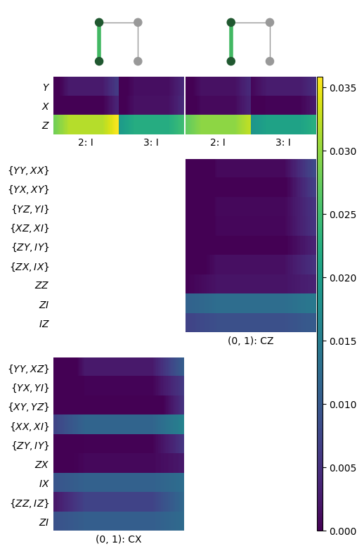
KNR estimates are no different than any other estimate and can be extracted using any of the methods outlined in earlier sections. For reference, one estimate object is constructed for every marginal distribution. For example, one estimate object might contain errors for I, X, Y, and Z for some particular single-qubit subsystem. In the heatmap, these appear as colums of sub-blocks, possibly with some entries missing if they are below the cutoff.
However, you might also be interested in extracting the numbers in an order exactly
as shown in the heatmap. First note, as seen in this example, that these heatmaps need
not be rectangular; differing degeneracies across gates can cause discrepancies in the
y-axis labels. However, we can access sub-rectangles of data using the class
KnrDataTable, which is used by the heatmap to
organize data, and can also be used by you.
[20]:
table = tq.estimate.KnrDataTable(fit)
# if necessary, set the truncation level, which will affect the amount of data shown
table.set_truncation(0)
If we access the top-left cell of data, we see that it has 3 rows for the three Pauli errors, and two columns, one for each idling subsystem.
[21]:
# access the top-left cell seen in the figure
table.get_cell(0, 0)
[21]:
Cell(mean=array([[3.18950683e-02, 2.21506894e-02],
       [2.41278228e-05, 1.62147007e-03],
       [2.62193321e-03, 1.32192012e-03]]), std=array([[0.00201139, 0.0014048 ],
       [0.00201139, 0.0014048 ],
       [0.00201139, 0.0014048 ]]), subcycles=[{(2,): Gate.id}, {(3,): Gate.id}])
[22]:
# access the exterior x-axis information of the first column
table.col_info[0]
[22]:
Col(name='', cycles=(Cycle((0, 1): Gate.cx),), twirl=Twirl({(0,): 'P', (1,): 'P', (2,): 'P', (3,): 'P'}, dim=2))
[23]:
# access the exterior y-axis information of the top row
table.row_info[0]
[23]:
Row(sort_key=(False, 1, (1,)), degens=[(('Z',),), (('X',),), (('Y',),)], param_names=['e__Z', 'e__X', 'e__Y'], latex=['$e_{Z}$', '$e_{X}$', '$e_{Y}$'])
Download
Download this file as Jupyter notebook: estimate_collections.ipynb.