Download
Download this file as Jupyter notebook: rcal_example.ipynb.
Example: Running Readout Calibration
This example illustrates how to generate readout calibration (RCAL) circuits and use them to correct readout errors in other circuits.
The make_rcal() method produces a set of circuits that prepare both
the ground state (through application of identity gates) and excited states
(through the application of bitflip or \(X\) gates in the case of qubits, or their
multi-dimensional equivalent in the case of qudits). The relative frequency with which
the ground and excited states are measured are used to estimate state-dependent
readout errors.
In this example we use the built-in Simulator to execute the
RCAL circuits, but the same procedure can be followed for circuits that are run on
hardware.
Readout Calibration in Qubits
The code below generates RCAL circuits for two qubits (labelled 0 and 1),
populates their results using a simulator with readout error, and displays the
resulting state probabilities in the form of confusion matrices.
[2]:
import trueq as tq

# generate RCAL circuits to measure the readout errors on qubits [0, 1]
circuits = tq.make_rcal([0, 1])

# display the circuits
circuits[0]
[2]:
|
Circuit
|
||
|
|
(0):
Gate.x
|
(1):
Gate.x
|
|
1
|
(0):
Meas()
|
(1):
Meas()
|
[3]:
circuits[1]
[3]:
|
Circuit
|
||
|
|
(0):
Gate.id
|
(1):
Gate.id
|
|
1
|
(0):
Meas()
|
(1):
Meas()
|
Next, we initialize a simulator with a 20% readout error on both qubits:
[4]:
sim = tq.Simulator().add_readout_error(0.2)

# run the circuits on the simulator to populate their results
sim.run(circuits, n_shots=1000)
We can analyze and fit the results by calling the
fit() method that produces the following output:
[5]:
circuits.fit()
[5]:
|
RCAL
Readout Calibration
|
Confusion |
| (0,) |
P(0 | 0) = 0.806 P(1 | 1) = 0.800
|
| (1,) |
P(0 | 0) = 0.796 P(1 | 1) = 0.795
|
Here, \(P(A|B)\) are conditional probabilities that denote the probability that we are measuring state \(A\) when we expect to have state \(B\) prepared. When you hover over each row in the table above it displays the confusion matrices of the outcomes, that is, the probabilities \(P(0|0), P(0|1), P(1|0)\) and \(P(1|1)\) arranged in matrix form. Given that we simulated these circuits with a 20% readout error, we observe a more or less 80/20 split in probabilities on the diagonal and the off-diagonal elements.
Readout Calibration in Qudits
The make_rcal() function can be used for qudits in exactly the same
way as for qubits. The qudit dimension determines how many circuits are needed to
estimate the error on all states, because there are more computational basis states
for higher-dimensional systems and therefore more conditional probabilities to
measure.
In this example we consider qutrits, that is qudits of dimension three, by setting
the set_dim() parameter to 3. Higher-dimensional qudits
can be analyzed in the same fashion.
For a qutrit, make_rcal() generates three circuits that prepare the
ground state on each qudit by applying identity gates, the first excited state by
applying \(X\) gates, and the second excited state by applying \(X^2\) gates
to each qudit.
As before, we consider a system of two qutrits (labelled 0 and 1) and start
by generating those circuits:
[6]:
tq.settings.set_dim(3)

circuits = tq.make_rcal([0, 1])

# display the circuits
circuits[0]
[6]:
|
Circuit
|
||
|
|
(0):
Gate.x3pow2
|
(1):
Gate.x3pow2
|
|
1
|
(0):
Meas()
|
(1):
Meas()
|
[7]:
circuits[1]
[7]:
|
Circuit
|
||
|
|
(0):
Gate.x3
|
(1):
Gate.x3
|
|
1
|
(0):
Meas()
|
(1):
Meas()
|
[8]:
circuits[2]
[8]:
|
Circuit
|
||
|
|
(0):
Gate.id3
|
(1):
Gate.id3
|
|
1
|
(0):
Meas()
|
(1):
Meas()
|
Next, we simulate the outcome of these circuits with a 20% readout error on both qutrits and fit the results:
[9]:
sim = tq.Simulator().add_readout_error(0.2)
sim.run(circuits, n_shots=1000)

estimate = circuits.fit()
estimate
[9]:
|
RCAL
Readout Calibration
|
Confusion |
| (0,) |
P(0 | 0) = 0.798 P(1 | 1) = 0.803 P(2 | 2) = 0.794
|
| (1,) |
P(0 | 0) = 0.796 P(1 | 1) = 0.783 P(2 | 2) = 0.799
|
And just as in the qubit case, when hovering over this table you can again inspect the confusion matrices that now have a dimension of \(3\times3\) and contain all the conditional probabilities \(P(0|0), P(0|1), P(0|2), P(1|0) \dots P(2|2)\).
Applying the Correction
The estimate returned by the RCAL protocol upon calling the
fit() method is an
RCalEstimate instance that can be used to apply a
correction to a different set of results that were obtained under the same readout
error. For this, we can call the
apply_correction() method that inverts the
confusion matrices and multiplies them onto the corresponding indices of the results
that we wish to correct.
For example, consider the following two-qutrit circuit with a Fourier or \(F\) gate (the generalized version of the Hadamard gate for higher qudit dimensions) on the first qutrit followed by a \(CX\) gate on both:
[10]:
circuit = tq.Circuit([{0: tq.Gate.f3}, {(0, 1): tq.Gate.cx3}])
circuit.measure_all()

circuit.draw()
[10]:
In the absence of readout errors, this circuit should produce an equal superposition
between the the states 00, 11 and 20. However, when we simulate this
circuit with the noisy simulator from above, the actual results differ. But
using the RCalEstimate we obtained from the calibration,
we can correct those results using the
apply_correction() method:
[11]:
results = sim.sample(circuit, n_shots=1000)

tq.visualization.plot_results(
    results,
    estimate[0].apply_correction(results),
    labels=["Bare Circuit", "With Readout Calibration"],
)
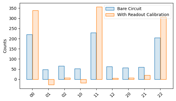
Note that the linear transformation used to correct the readout results can yield negative-valued outputs in the histogram, which can be interpreted as zero outputs.
Automatic Correction
The correction we applied manually in the example above can also be automated. If you
are using a CircuitCollection that also contains RCAL circuits,
then that information will be used automatically to apply readout correction to your
circuits when you call fit() or
plot().
The code below illustrates this for SRB (Streamlined Randomized Benchmarking) circuits executed on a noisy simulator with readout error. It also shows how you can view the results with and without readout correction being applied. For simplicity, we switch our focus back to qubits but the example below works for qudits as well.
[12]:
tq.settings.set_dim(2)

# generate RCAL circuits to measure the readout errors on three qubits [0, 1, 2]
circuits = tq.make_rcal([0, 1, 2])

# generate SRB circuits to simultaneously characterize a single qubit [0] and
# a pair of qubits [1, 2] with 30 circuits for each random cycle in [4, 32, 64]
circuits.append(tq.make_srb([[0], [1, 2]], [4, 32, 64], 30))

# initialize a noisy simulator with a 10% readout error
sim = tq.Simulator().add_stochastic_pauli(px=0.01).add_readout_error(0.1)

# RCAL generally needs more shots than the other protocols because it is estimating
# an absolute value rather than a decay over randomizations, thus in this simulation
# we use different numbers of shots for RCAL and SRB to populate their results
sim.run(circuits.subset(protocol="RCAL"), n_shots=1000)

# to simulate the SRB circuits, we create a subset that contains all circuits except
# those from RCAL, which we can achieve by using square brackets in our syntax:
sim.run(circuits.subset(protocol=["RCAL"]), n_shots=50)

# plot the exponential decay with readout correction,
# where each expectation value (dot) has been compensated
circuits.plot.raw()
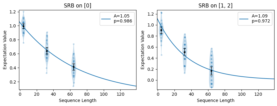
To avoid performing readout correction during analysis, we can remove all RCAL
circuits from the collection before calling plot().
Notice that the y-intercept is now lower than in the plot above:
plot the exponential decay without readout correction
[13]:
circuits.subset(protocol="SRB").plot.raw()

Download
Download this file as Jupyter notebook: rcal_example.ipynb.