Download
Download this file as Jupyter notebook: srb_example.ipynb.
Example: Running SRB
These examples demonstrate how to use SRB, the most basic QCVV protocol, to estimate the process infidelity of a single-qudit or two-qudit gateset [1] .
Getting started
The simplest thing we can do is run SRB on a single qubit. Qubits are labeled by
non-negative integers, and here we target qubit 0. We choose to use sequence lengths
[4, 30, 50], and, by default, 30 random circuits are generated per sequence
length. Below, we display the first circuit where the 4 random Clifford gates can be
seen, plus a fifth gate which is the product of their inverses and a random Pauli
matrix, where the additional Pauli matrix is introduced to make the fit more robust.
The empty cycles with non-zero markers delimit the random Cliffords, and more
generally, in other protocols like make_cb() and
make_irb(), contain interleaved cycles of interest.
[2]:
import trueq as tq
import trueq.simulation as tqs

circuits = tq.make_srb(0, [4, 30, 50])
circuits[0]
[2]:
|
Circuit
|
|
|
1
|
(0):
Gate.cliff11
|
|
2
|
(0):
Gate.id
|
|
3
|
(0):
Gate.x
|
|
4
|
(0):
Gate.sy
|
|
5
|
(0):
Gate.cliff22
|
|
6
|
(0):
Meas()
|
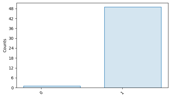
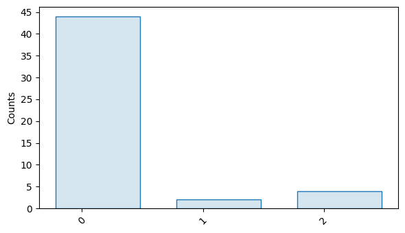
Next, we simulate each of the circuits with the built-in simulator. We can see the bitstring counts of the first circuit below.
[3]:
tq.Simulator().add_overrotation(0.04).add_depolarizing(0.01).run(circuits)
circuits[0].results.plot()
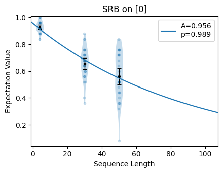
It is important to look at the decay curve to verify that appropriate sequence lengths
were chosen. The most informative sequence length to measure occurs around
\(m=1/(1-p)\) where the decay is \(y=Ap^m\). If \(A\approx 1\) and
\(p\approx 1\), then this corresponds to \(y\approx1/e\approx0.37\).
Therefore, in this example, our sequence lengths are a bit too short, and [4, 70]
would, in retrospect, have been more appropriate.
[4]:
circuits.plot.raw()
Finally, we can look at the values of the estimate:
[5]:
circuits.fit()
[5]:
|
SRB
Streamlined Randomized Benchmarking
|
Cliffords
(0,)
|
|
${e}_{F}$
The probability of an error acting on the targeted systems during a random gate.
|
8.3e-03 (8.9e-04)
0.008284486241839556, 0.0008885775122893031
|
|
${p}$
Decay parameter of the exponential decay $Ap^m$.
|
9.9e-01 (1.2e-03)
0.9889540183442139, 0.0011847700163857375
|
|
${A}$
SPAM parameter of the exponential decay $Ap^m$.
|
9.6e-01 (1.8e-02)
0.955731935790638, 0.017864898883745973
|
Isolated vs. Simultaneous SRB
The core function make_srb() generates a circuit collection that
implements simultaneous SRB, where gates are placed on all specified qubits of a
quantum device within each circuit. Different random gates are independently chosen
during each cycle. Qubit labels are entered into its first argument and specify which
qubits are acted on simultaneously. You can choose which qubits get single-qubit
twirls, and which qubits get two-qubit twirls, by nesting the qubit labels
appropriately; see the following examples.
[6]:
# simultaneous single-qubit RB on qubits 0 and 1; 60 circuits total
circuits = tq.make_srb([0, 1], [4, 100], 30)

# isolated single-qubit RB on qubits 0 and 1; 120 circuits total
circuits = tq.make_srb([0], [4, 100], 30).append(tq.make_srb([1], [4, 100], 30))

# two-qubit RB on 0 and 1, simultaneous with single-qubit RB on 2; 60 circuits total
circuits = tq.make_srb([[0, 1], 2], [4, 100], 30)
The invocations above all use two sequence lengths (the number of random gate cycles
in a circuit), 4 and 100, and produce 30 random circuits per sequence length. Note
that specifying qubit labels [0, 1, 2] is a convenient short-hand for
[[0], [1], [2]]. This imples, for example, that [[0,1]] has a much different
meaning than [0,1].
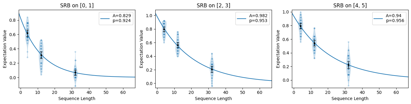
Isolated SRB
In isolated SRB, we characterize qubits or qubit-pairs one at a time with disjoint experiments. This is done to assess gate quality on a small subregister in the context of an idling environment. In this example, we build a single circuit collection to estimate the average gate infidelity of three pairs on a 6 qubit device.
[7]:
# generate a circuit collection
circuits = tq.CircuitCollection()
for pair in [[0, 1], [2, 3], [4, 5]]:
    circuits += tq.make_srb([pair], [4, 12, 32])
Next, we transpile the circuits into native gates and simulate them.
[8]:
# Initialize a simulator
sim = tq.Simulator().add_overrotation(0.01, 0.02)
sim.add_stochastic_pauli(px=0.01, match=tqs.LabelMatch((0, 1)))
sim.add_stochastic_pauli(pz=0.005, match=tqs.LabelMatch((2, 3, 4, 5)))

# initialize a transpiler into native gates (U3 and CNOT)
cnot_factory = tq.config.GateFactory.from_matrix("cnot", tq.Gate.cnot.mat)
config = tq.Config(factories=[tq.config.u3_factory, cnot_factory])
t = tq.Compiler.from_config(config)

# transpile and simulate
circuits = t.compile(circuits)
sim.run(circuits)
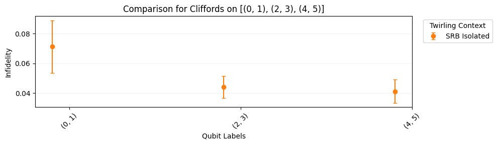
Plot the results.
[9]:
circuits.plot.raw([[0, 1], [2, 3], [4, 5]])
circuits.plot.compare_rb()
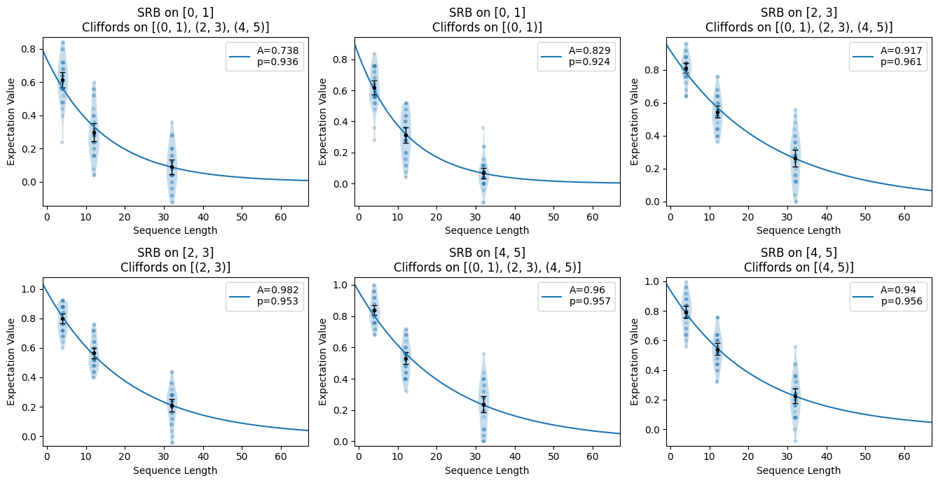
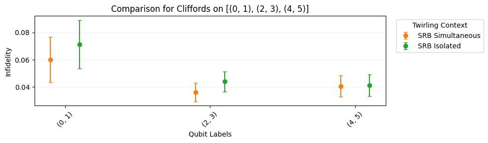
Simultaneous SRB
In simultaneous SRB, we characterize qubits or qubit-pairs in a single set of experiments. This captures crosstalk between these subsystems which is usually not present when other qubits are idle. In this example, we add more circuits to the circuits from the previous section.
[10]:
# add simultaneous circuits to our old collection
simul_circuits = t.compile(tq.make_srb([[0, 1], [2, 3], [4, 5]], [4, 12, 32]))
circuits += simul_circuits
sim.run(simul_circuits)

# plot the results
circuits.plot.raw([[0, 1], [2, 3], [4, 5]])
circuits.plot.compare_rb()
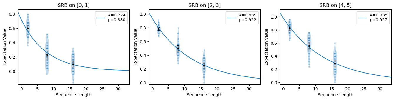
Changing the Twirling Group Gateset
The above examples characterize the average gate fidelity of the Clifford group, which is historically by far the most common group to use. However, any unitary 2-design will suffice, and so for SRB, the other notable choice is the set of all unitaries sampled using the Haar measure. We make this alternate choice below.
[11]:
su_circuits = tq.make_srb(tq.Twirl("U", [[0, 1], [2, 3], [4, 5]]), [2, 8, 16])
su_circuits = t.compile(su_circuits)
sim.run(su_circuits)
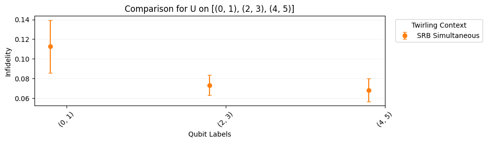
Our native gates here are still CNOT and U3. It takes on average 1.5 CNOTs to synthesize a two-qubit Clifford gate, but it almost always takes 3 CNOTs to synthesize a Haar-random two-qubit unitary group. Thus we see higher error rates than in the section above.
Simulate and plot the results.
[12]:
su_circuits.plot.raw([[0, 1], [2, 3], [4, 5]])
su_circuits.plot.compare_rb()
SRB with Qudits
The examples above generalize to qudits of higher dimensions and we can use the exact same syntax to generate and simulate the circuits and subsequently analyze their results. Let’s go through an example with a single qutrit:
[13]:
tq.settings.set_dim(3)

circuits = tq.make_srb(0, [4, 32, 64])

# display a sample circuit
circuits[0]
[13]:
|
Circuit
|
|
|
1
|
(0):
Gate(
|
|
2
|
(0):
Gate(
|
|
3
|
(0):
Gate(
|
|
4
|
(0):
Gate(
|
|
5
|
(0):
Gate.f3
|
|
6
|
(0):
Meas()
|
Next, we simulate each of the circuits with the built-in simulator and display a sample bitstring result:
[14]:
tq.Simulator().add_overrotation(0.04).add_depolarizing(0.02).run(circuits)

circuits[0].results.plot()
The decay curve can be inspected using the plot()
method:
[15]:
circuits.plot.raw()
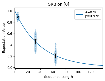
And similarly we can inspect the fit parameters:
[16]:
circuits.fit()
[16]:
|
SRB
Streamlined Randomized Benchmarking
|
Cliffords
(0,)
|
|
${e}_{F}$
The probability of an error acting on the targeted systems during a random gate.
|
2.1e-02 (1.3e-03)
0.021145009580573613, 0.0012815909107993097
|
|
${p}$
Decay parameter of the exponential decay $Ap^m$.
|
9.8e-01 (1.4e-03)
0.9762118642218547, 0.0014417897746492234
|
|
${A}$
SPAM parameter of the exponential decay $Ap^m$.
|
9.8e-01 (2.6e-02)
0.9833064258992447, 0.02645315098528627
|
Footnotes
Download
Download this file as Jupyter notebook: srb_example.ipynb.