---

Download

Download this file as Jupyter notebook: knr_example.ipynb.

Example: Running KNR

K-body noise reconstruction (KNR) is an error diagnostic protocol that provides a detailed error profile of a cycle of interest. In this example, we will see how to generate and run KNR circuits, and how to interpret the results. First, let’s choose a cycle to benchmark:

import numpy as np
import trueq as tq
import trueq.math as tqm
import trueq.simulation as tqs

# define the cycle to benchmark using KNR
cycle_of_interest = tq.Cycle({(0, 1): tq.Gate.cx, 2: tq.Gate.z})

This cycle is to be implemented on a quantum processor. For the sake of this example, the device in question will consist of a Simulator. To avoid confusion, we will name it device. Our device will be a minimalistic 3-qubit processor. Now, let’s introduce a stochastic error map to our cycle_of_interest:

# define some simple 3-qubit errors, together with their probability
error_profile = {
    #  no error with prob 88%
    "III": 0.88,
    # IXI error with prob  1%
    "IXI": 0.01,
    # XII error with prob  3%
    "XII": 0.03,
    # IXX error with prob  6%
    "IXX": 0.06,
    # ZXZ error with prob  2%
    "ZXZ": 0.02,
}

# define Kraus operators based on the above error profile
kraus_list = [
    np.sqrt(prob) * tqm.Weyls(pauli, dim=2).herm_mat
    for pauli, prob in error_profile.items()
]

# instantiate a superoperator based on the Kraus operators
superop = tqm.Superop.from_kraus(kraus_list)

# instantiate a device simulator based on the above error profile
device = tqs.Simulator()
device.add_cycle_noise(
    # the 3-qubit error map is applied to qubits 0, 1, and 2
    {(0, 1, 2): superop},
    # the error map is only applied to the cycle of interest
    match=tqs.CycleMatch(cycle_of_interest),
    # the error map occurs before the cycle of interest
    cycle_offset=-1,
)

<trueq.simulation.simulator.Simulator at 0x7fd27b3e5eb0>

Now that the device has been instantiated, let’s try to learn the error profile of the cycle_of_interest. For this, we will generate KNR circuit collections. An important parameter when generating KNR circuits is subsystems. To understand this parameter, let’s first identify the gate suppports of our cycle of interest, which are \((0,1)\) and \((2)\). If subsystems=1, the KNR protocol will yield marginal error probabilities for each gate support in the cycle of interest.

Given our example, if we look at qubit \(2\), which is a gate support for the cycle of interest, we should expect to see an \(X\) error with probability \(6\%\), and a \(Z\) error with probability \(2\%\). If we look at the gate support \((0,1)\), we should expect to see an \(XI\) error with probability \(3\%\), a \(ZX\) error with probability \(2\%\), and a \(IX\) error with probability \(7\%\). To obtain the \(7\%\) value, we added the probabilities of \(IXI\) and \(IXX\), which both yield an \(IX\) error for the support \((0,1)\) (this is the marginal probability). These are indeed the reconstructed probabilities:

# generate KNR circuits to benchmark the cycle, targeting only single gate supports
knr_circuits_1 = tq.make_knr(
    cycle_of_interest, n_random_cycles=[4, 10], n_circuits=30, subsystems=1
)

# run the circuits on the device
device.run(knr_circuits_1)

# plot the reconstructed error profile with subsystems=1:
layout = tq.visualization.Graph.linear(3, show_labels=True)  # specify the chip layout
knr_circuits_1.plot.knr_heatmap(layout)  # plot the heatmap

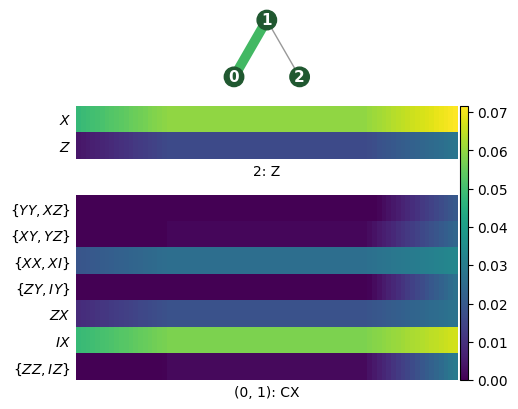
In the plot above, notice that the uncertainty for reconstructed error probabilities is seen in the variation of color in each cell. Some errors that are not included in the underlying error_profile might appear in dark purple due to the uncertainty of the estimates. These dark purple cells can be removed from the plot by simply changing the cutoff options (see the knr_heatmap API reference). Moreover, notice the label \(\{XX,XI\}\), which is associated with a probability of \(3\%\). This bracketed set of errors is short for “\(XX\) or \(XI\)" and indicates that KNR didn’t differentiate between the two and instead outputs the sum of their respective probability of occuring. \(XX\) and \(XI\) are then said to be “degenerate”. Here, we know from our construction that only \(XI\) could occur, but on an actual device where the noise model is unknown, we cannot learn the individual error probabilities in a degenerate set.

Advanced note: KNR degeneracies

Degeneracies are determined by the cycle of interest. Given a Clifford cycle of interest \(G\), the KNR degeneracies are determined by its Weyl orbits; the orbit of a Weyl operator \(W\) with respect to \(G\) is defined as

\[W^{\circlearrowright G}:= \{W, G(W), G^2(W), \cdots\}~.\]

For example, the orbit of \(XX\) given a \(CX\) gate is

\[\begin{split}XX^{\circlearrowright CX}&= \{XX, CX(XX)\} \\ &= \{XX, XI\}~.\end{split}\]

Aside from the \(\{XX, XI\}\) degeneracy, we might want to resolve our error profile further. Indeed, from the current experiment (i.e. with subsystems=1), we can’t know if some errors on different gate supports are correlated. For instance, we know that qubit \(2\) sees a \(Z\) error with probability of \(2\%\), and that the qubit pair sees a \(ZX\) error with probability of \(2\%\), but we didn’t learn if these errors occur at the same time or not (we know from our underlying error profile that they are perfectly correlated). To resolve the error correlations between any two gate supports, we can simply choose a KNR circuit collection with subsystems=2:

# generate KNR circuits to benchmark the cycle, targeting all pairs of gate supports
knr_circuits_2 = tq.make_knr(
    cycle_of_interest, n_random_cycles=[4, 10], n_circuits=30, subsystems=2
)

# run the circuits on the device
device.run(knr_circuits_2)

# plot the reconstructed error profile with subsystems=2:
knr_circuits_2.plot.knr_heatmap(layout)  # plot the heatmap

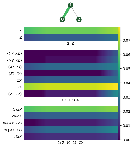
Notice that this experiment yields marginal error probabilities for all pairs of gate supports. Since our cycle only contained a pair of gate supports (namely \((0,1)\) and \(2\)), the above plot shows a complete reconstruction of the error profile.

Specifying which subsystems to probe

When the subsystems argument of make_knr() is an integer, it specifies the maximum number of gate-bodies whose correlated errors should be reported. For example, if the cycle is a CNOT on qubits \((0, 1)\) with idling qubits \(2\) and \(3\), then when subsystems=2, in addition to reporting single gate-body errors on each of the subsystems \((0, 1)\), \((2,)\), and \((3,)\), errors will also be reported on the gate-body pairs corresponding to \((0, 1, 2)\), \((0, 1, 3)\), and \((2, 3)\). In general, for subsystems=k, n-choose-k subsystems will be very large and require many circuits to reconstruct the errors.

To reduce experiment cost, the subsystems argument can be specified as a Subsystems object where subsystems to reconstruct are explicitly defined. In this example, we demonstrate how this approach can allow for a less costly reconstruction by exploiting knowledge of the system being characterized. Consider a linear array of qubits and a cycle of single-qubit gates with underlying \(ZZ\) couplings between adjacent qubits. Rather than reconstructing all combinations of \(2\) operations, we expect distant pairs, e.g. \((0, 4)\), to have no correlated errors and thus omit them.

# define the cycle of interest to benchmark
cycle_of_interest = tq.Cycle({range(5): tq.Gate.x})

# define the layout of our device
layout = tq.visualization.Graph.linear(5, show_labels=True)

# define the ZZ couplings in our device
error_profile = {
    "IIIII": 0.90,
    "ZZIII": 0.02,
    "IZZII": 0.01,
    "IIZZI": 0.03,
    "IIIZZ": 0.04,
}

kraus_list = [
    np.sqrt(prob) * tqm.Weyls(pauli, dim=2).herm_mat
    for pauli, prob in error_profile.items()
]

# instantiate a superoperator based on the Kraus operators
superop = tqm.Superop.from_kraus(kraus_list)

# instantiate a device simulator based on the above error profile
device = tqs.Simulator()
device.add_cycle_noise(
    {(0, 1, 2, 3, 4): superop},
    match=tqs.CycleMatch(cycle_of_interest),
    cycle_offset=-1,
)

# use from_cycle and nearest_neighbour methods to create subsystems to analyze
subsystems = tq.Subsystems.from_cycle(cycle_of_interest).nearest_neighbour(layout)
subsystems

Subsystems(((0,), (1,), (2,), (3,), (4,), (0, 1), (1, 2), (2, 3), (3, 4)))

By using the methods of the Subsystems class, we specified that we only want to reconstruct the errors on adjacent pairs of qubits when calling make_knr().

knr_circuits_1 = tq.make_knr(
    cycle_of_interest, n_random_cycles=[4, 10], n_circuits=30, subsystems=subsystems
)
device.run(knr_circuits_1)

# plot the reconstructed error profile on the specified subsystems:
knr_circuits_1.plot.knr_heatmap(layout)

# print the total number of circuits
knr_circuits_1.n_circuits

540

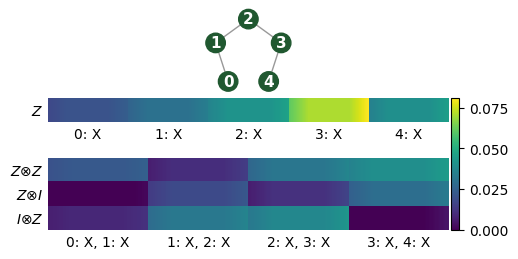
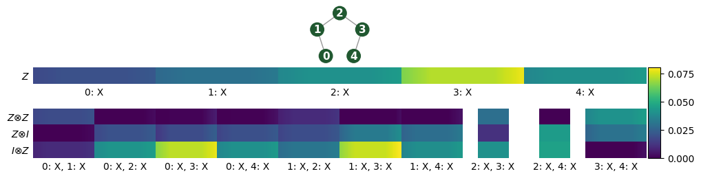
Comparing the above output with a call to make_knr() with subsystems=2, we note that we were able to perform the reconstruction with fewer circuits and omit information about the errors on uncoupled pairs.

knr_circuits_2 = tq.make_knr(
    cycle_of_interest, n_random_cycles=[4, 10], n_circuits=30, subsystems=2
)
device.run(knr_circuits_2)

# plot the reconstructed error profile with subsystems=2:
knr_circuits_2.plot.knr_heatmap(layout)

# print the total number of circuits
knr_circuits_2.n_circuits

1200

KNR with qudits

KNR seamlessly supports qudits. To see this, let’s recreate a similar example as above, but with qutrit instructions on a 2-qutrit processor:

# setting the register dimension to 3 (i.e. qutrits)
tq.settings.set_dim(3)

# define the cycle to benchmark using KNR
cycle_of_interest = {(0, 1): tq.Gate.cx3}

# define some simple error profile by pairing Weyl errors with corresponding
# probabilities
error_profile = {
    #  no error with prob 88%
    "W00W00": 0.88,
    # X3.I3 error with prob  2%
    "W10W00": 0.02,
    # X3.Z3 error with prob  8%
    "W10W01": 0.08,
    # I3.X3 error with prob  2%
    "W00W10": 0.02,
}

# define Kraus operators based on the above error profile
kraus_list = [
    np.sqrt(prob) * tqm.Weyls(weyl).mat for weyl, prob in error_profile.items()
]

# instantiate a superoperator based on the Kraus operators
superop = tqm.Superop.from_kraus(kraus_list)

# instantiate a device simulator based on the above error profile
device = tqs.Simulator()
device.add_cycle_noise(
    # the 3-qutrit error map is applied to qutrits 0, 1, and 2
    {(0, 1): superop},
    # the error map is only applied to the cycle of interest
    match=tqs.CycleMatch(cycle_of_interest),
    # the error map occurs before the cycle of interest
    cycle_offset=-1,
)

<trueq.simulation.simulator.Simulator at 0x7fd27a71ee80>

Now that the device has been instantiated, let’s try to learn the error profile of the cycle_of_interest:

# generate KNR circuits to benchmark the cycle, targeting only single gate supports
knr_circuits = tq.make_knr(
    cycle_of_interest, n_random_cycles=[6, 9, 12], n_circuits=30, subsystems=1
)

# run the circuits on the device
device.run(knr_circuits)

# plot the reconstructed error profile with subsystems=1:
layout = tq.visualization.Graph.linear(2, show_labels=True)  # specify the chip layout
knr_circuits.plot.knr_heatmap(layout)  # plot the heatmap

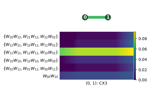
Notice that for this cycle, some degeneracy orbits contain \(3\) Weyl operators. This observation is expected as tq.Gate.cx3 has a cyclicity of \(3\).

Advanced Usage: Specifying a custom twirl to diagnose idle qubits

For full-system diagnostics, we are often interested in the error that occurs on idling qubits. This can be done by specifying a custom Twirl that includes the labels of the idle qubits.

For example, let’s consider a cycle with a \(CX\) gate on qubits 0 and 1 and an additional, idling qubit with label 2. We instantiate a simulator that adds a stochastic \(Z\) error to the idling qubit and define a twirl on all three qubit labels:

tq.settings.set_dim(2)

cycle_of_interest = tq.Cycle({(0, 1): tq.Gate.cx})

twirl = tq.Twirl("P", (0, 1, 2))

circuits = tq.make_knr(
    cycle_of_interest, twirl=twirl, n_random_cycles=[4, 10], n_circuits=30, subsystems=1
)

sim = tq.Simulator().add_stochastic_pauli(pz=0.1, match=tq.simulation.LabelMatch(2))

sim.run(circuits)

layout = tq.visualization.Graph.linear(3, show_labels=True)
circuits.plot.knr_heatmap(layout)

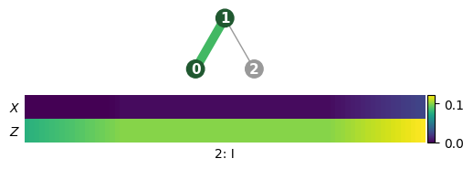
As expected, the resulting error map is dominated by a single-qubit \(Z\) errors on qubit 2, whereas there is no significat error observed on the \(CX\) gate.

circuits.fit()

True-Q formatting will not be loaded without trusting this notebook or rerunning the affected cells. Notebooks can be marked as trusted by clicking "File -> Trust Notebook".

One or more estimates with probabilities below the cutoff threshold have been omitted.

KNR Estimates K-body Noise Reconstruction	Paulis (0, 1): Gate.cx Cycle: (0, 1): Gate.cx Twirl: Paulis on [0, 1, 2]
	(2,) : Gate.id Cycle: (0, 1): Gate.cx
Z	1.0e-01 (1.1e-02) Subcycle: (2,): Gate.id Error Type: Z Error Probability (std): 0.09961917037745716 (0.01129578315667583)
X	3.5e-03 (1.1e-02) Subcycle: (2,): Gate.id Error Type: X Error Probability (std): 0.0034546652619686924 (0.01129578315667583)

---

Download

Download this file as Jupyter notebook: knr_example.ipynb.