Example: Quantum Circuits with Qudits

Quantum systems used for quantum computing contain quantized energy levels which can be used to define computational states. Most quantum computing devices follow the standard classical convention of using a two-level system with basis states labeled by 0 and 1, that is a canonical qubit.

Since quantum systems generally have more than two energy levels available, the restriction to only two of them does not allow the quantum device to fully leverage the available state space. Additionally, the presence of unused levels can lead to loss of information as the state can “leak” into unused energy levels. For this reason, some hardware developers choose to design their quantum computing devices to use more than the standard two levels. In these cases, the multi-level unit is referred to as a qudit. Many of our tutorials refer only to qubits for simplicity. However, our protocols apply more generally to qudits.

The dimension of a qudit refers to the number of energy levels used to store information. True-Q™ supports qudit systems of dimensions 2, 3, 5 and 7. These prime dimensions are compatible with the stabilizer formalism and measurements for these dimensions produce single-digit outputs.

In this tutorial, we provide a basic introduction to qudits and show how to start creating True-Q™ circuits for qudits. We direct users to Advanced Qudit Framework for a more in-depth introduction to the mathematical framework used to model qudit computations and an overview of the classes used to represent the operations defined for that framework.

We define the computational basis of a qudit to be an orthogonal set of states, each of which corresponds to a single energy level,

\[\{\ket{0}, \ket{1}, ..., \ket{d-1}\}.\]

A qudit state \(\ket{\psi}\) can then be expressed as a linear combination of these basis states,

\[\ket{\psi}=\sum_{a=0}^{d-1}c_a(\psi)\ket{a},\]

where \(c_a(\psi)\) are constants.

Using Qudits in True-Q™

Qudit circuits can be constructed in the same way as regular qubit circuits, and in fact most of the True-Q™ tools work with no or very minor syntax modifications for qudits.

We provide gate aliases for standard qudit gates that follow the same naming convention as the qubit gates but with the dimension attached to their name, e.g. the alias tq.Gate.x3 represents a qutrit \(X\) gate. Using these aliases, defining circuits is straight-forward:

We can specify the qudit dimension we want to work in by setting the global dimensional parameter:

[2]:

import trueq as tq

# set the global dimension to 3
tq.settings.set_dim(3)

To start off, let’s define a simple circuit for a two-qutrit system that consists of a single-qutrit \(X\) gate, a single-qutrit \(F\) or Fourier gate (the higher-dimensional generalization of the Hadamard gate), and a two-qutrit controlled-\(X\) gate. Note that we define gate aliases for standard qudit gates following the same convention of qubit gates but with the dimension appended (e.g. the alias tq.Gate.x3 represents a qutrit \(X\) gate).

[3]:

cycle1 = tq.Cycle({(0,): tq.Gate.f3, (1,): tq.Gate.x3})
cycle2 = tq.Cycle({(0, 1): tq.Gate.cx3})

circuit = tq.Circuit([cycle1, cycle2])
circuit.measure_all()

circuit.draw()

[3]:

As in the qubit case, we can use the Simulator to simulate the outcomes of this circuit:

[4]:

sim = tq.Simulator()
sim.run(circuit)

circuit.results.plot()

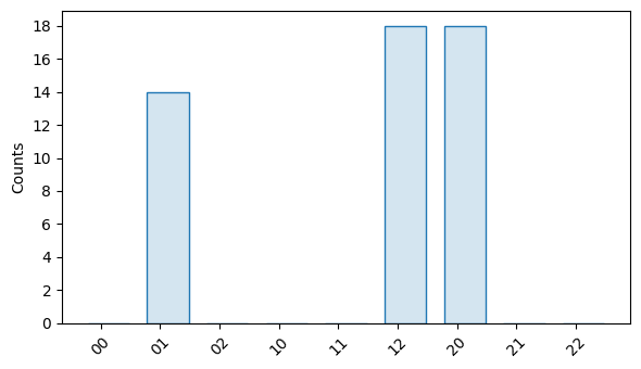
../../_images/guides_fundamentals_qudit_intro_7_0.png

Notice that since the circuit we ran acts on 2 qutrits, the results are in \(\mathbb{Z}_3^2 = \{00, 01, ..., 22\}\) because the computational state space for a single \(d\)-dimensional qudit spans \(\mathbb{Z}_d=\{0, 1, ... d-1\}\).

Qudit Protocols

As mentioned above, our True-Q™ protocols generalize seamlessly to qudits of dimension larger than \(2\). For example, take a look at how the following protocols work for qudits:

Download

Download this file as Jupyter notebook: qudit_intro.ipynb.