The building blocks of quantum algorithms are gates, cycles, and circuits. A gate is
an operation that can act on one or more qudits. A cycle is a single step of an
algorithm, which contains gates and qudit labels specifying which qudits those gates
act on. A circuit is a sequence of cycles that ultimately is run on a device. In this
tutorial, we focus on 2-level systems, or qubits. A simple diagram of a circuit
acting on qubits is included below to show how these building blocks fit together.
A quantum circuit represented in the True-Q™ interface. The horizontal
lines denote the qubits, labeled here from 0 to 2, and the gates applied
to each qubit are represented by labeled boxes. Time moves from left to
right in this picture, so the Cycle #1 acts first and applies a Hadamard
(or \(H\)) gate to each of the qubits. Next, Cycle #2
applies a \(CZ\) gate to qubits 0 and 1. Then Cycle #3 applies a
\(CZ\) gate to qubits 0 and 3, and so on.
The circuit in the figure above creates the 3-qubit GHZ state,
\(\frac{1}{\sqrt{2}}(\ket{000}+\ket{111})\).
We now show how to make the corresponding GHZ circuit in True-Q™.
The first step in constructing a circuit is generally to define its gates. In this
example however, we can simply use True-Q™’s built-in gates to implement the circuit.
You can refer to Example: Configuring Native Gates for details on
True-Q™’s methods for gate construction; these will be helpful when constructing
gates that are less standard. The two gates we will use are the Hadamard gate
(available through the trueq.Gate.h object) and the controlled-\(Z\) gate
(trueq.Gate.cz).
Next, we can construct the cycles that make up this circuit as follows:
In the above code snippet, the qubits are labeled 0 through 2 and the qubits each gate
acts on in a given cycle are specified before the gate is given as (labels):gate.
Next we construct the circuit as a chronologically ordered list of cycles:
[3]:
circuit=tq.Circuit([cycle1,cycle2,cycle3,cycle4])
To generate a visual representation of this circuit as we have seen above, we can call
the draw() method:
[4]:
circuit.draw()
[4]:
This generates an interactive circuit visualization that allows you to inspect the
circuit’s individual operations by hovering over the gates with your mouse.
If we want to perform measurements at the end of the circuit, we can append a cycle of
measurements using the measure_all() method:
To inspect the action that a certain circuit has on a given number of qubits, we can
use True-Q™’s built-in simulator to simulate the results. We can initialize an ideal
simulator as follows:
[6]:
sim=tq.Simulator()
The simulator assumes the initial state is \(\ket{0}^{\otimes n}\) by default, but
can be customized to have a different initial state. Noise models can also be added to
the simulator to investigate how circuits behave when run on error-prone quantum
devices. By calling the run() method, you can simulate the
circuit on the simulator we initialized above:
[7]:
sim.run(circuit,n_shots=100)
The n_shots keyword specifies how many times we want the results to be sampled
from the final quantum state after running this circuit. If we set it to infinity,
(e.g. float("inf") or numpy.inf`) then we obtain the exact simulated
probabilities.
When a circuit is run on a simulator, the results are written to the
circuit.result attribute. To view them, we can can simply print them out:
[8]:
circuit.results
[8]:
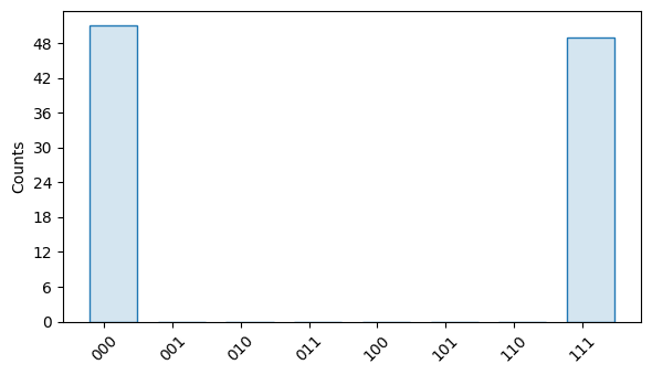
Results({'000': 51, '111': 49})
We expect the output to contain only 000 and 111 since these are the only
basis states that are populated in a GHZ state, and they should occur with roughly
equal probability. However, since each run has a 50/50 probability of returning either
result, the results will not necessarily be divided evenly between the two outcomes.
In addition to printing the results of a simulation, we can also visualize them
using True-Q™’s plotting capabilities. To generate a simple histogram, you can call
the plot() method: