---

Download

Download this file as Jupyter notebook: rc_simple_intro.ipynb.

Example: Running Randomized Compiling

This example provides a short demonstration of True-Q™’s randomly_compile() function and how it can be used to generate a set of randomly compiled circuits from a single input circuit, while implementing the same unitary as the original circuit. For more background information, check out our Randomized Compiling (RC) user guide page.

Note

Randomized compiling produces a new circuit collection after each call, so the output of this example will be different if it’s executed again.

Generating randomly compiled circuits

We begin by creating a simple two-qubit circuit with alternating cycles:

import numpy as np
import trueq as tq

cycle1 = {0: tq.Gate.h}
cycle2 = {(0, 1): tq.Gate.cz}
cycle3 = {1: tq.Gate.h}

circuit = tq.Circuit([cycle1, cycle2, cycle3] * 3)
circuit.measure_all()
circuit.draw()

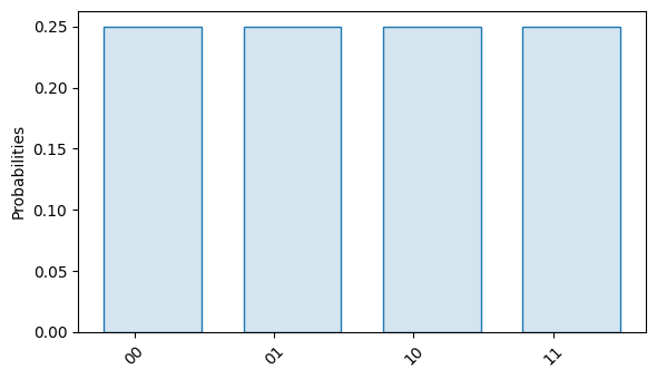
This circuit produces an equal superposition state of all four possible two-qubit states, as a quick simulation with our built-in Simulator shows:

sim = tq.Simulator()
ideal_result = sim.sample(circuit, n_shots=np.inf)
ideal_result.plot()

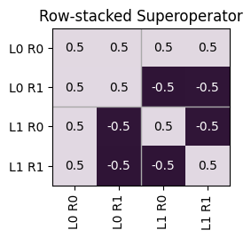
We can also inspect the operator that this circuit is implementing:

circuit_operator = sim.operator(circuit).mat()
tq.math.Superop(circuit_operator).plot_rowstack()

To generate a set of randomly compiled versions of this circuit, we call the randomly_compile() function and pass our circuit as argument, together with the desired number of compilations:

n_compilations = 30
rc_circuits = tq.randomly_compile(circuit, n_compilations=n_compilations)

This function returns a CircuitCollection of 30 randomized versions of our original circuit. For example, the first circuit in this collection looks like this:

rc_circuits[0].draw()

We can verify that this circuit (as well as every other circuit in this collection) implements the same operation (up to a global phase) as our original circuit by again inspecting the circuit operator:

rc_circuit_operator = sim.operator(rc_circuits[0]).mat()
tq.math.Superop(rc_circuit_operator).plot_rowstack()

For a phase-insensitive comparison, we can calculate the process infidelity between these two operators. The process infidelity is a metric for how different two operations are; an infidelity of zero means they are equivalent up to a phase. We can use the built-in proc_infidelity() function for this:

tq.math.proc_infidelity(circuit_operator, rc_circuit_operator)

-8.881784197001252e-16

Finally, when we sample from the final state’s probability distribution every circuit yields the same result:

for rc_circuit in rc_circuits:
    assert tq.utils.dicts_close(sim.sample(rc_circuit, n_shots=np.inf), ideal_result)

Measuring RC performance

To test how well Randomized Compiling works in practice, let’s walk through a short simulation of the circuit above with a noisy simulator and look at how the RC circuits perform relative to the bare circuit.

First, we create a simulator with an overrotation error as the noise source and simulate the outcomes of the bare circuit under this noise model:

noisy_sim = tq.Simulator().add_overrotation(single_sys=0.1, multi_sys=0.1)
noisy_result = noisy_sim.sample(circuit, n_shots=np.inf)
noisy_result.plot()

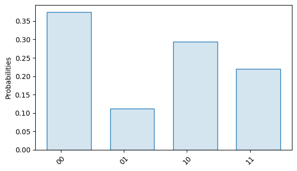
Note that we are no longer seeing the equal superposition that the noise-free simulation produced.

Next, we simulate the randomly compiled circuits under the same noise model, and sum the outcomes over all circuits:

# run all circuits on the simulator
noisy_sim.run(rc_circuits, n_shots=np.inf)

# sum over the outcomes
rc_result = rc_circuits.sum_results()

# for plotting, we normalize the summed results to be between 0 and 1
rc_result.normalized().plot()

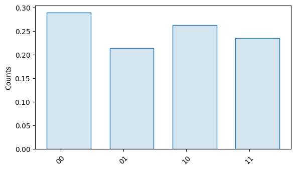
Under Randomized Compiling, the noisy simulation produces a result that is much closer to the noise-free simulation. In fact, we can use the trueq.Results.tvd() method of the Results class to quantify this difference:

bare_tvd = noisy_result.tvd(ideal_result)
rc_tvd = rc_result.normalized().tvd(ideal_result)

print("Noisy simulation without RC: {:.4f}".format(bare_tvd[0]))
print("Noisy simulation with RC: {:.4f}".format(rc_tvd[0]))

Noisy simulation without RC: 0.1686
Noisy simulation with RC: inf

Warning: divide by zero encountered in divide
         (/home/jenkins/workspace/release trueq/trueq/results.py:489)

The TVD, or Total Variation Distance is a measure for how far two probability distributions are apart. A value of zero means the distributions are equivalent.

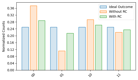
Finally, we can produce a visual summary of these results:

tq.visualization.plot_results(
    ideal_result,
    noisy_result,
    rc_result,
    labels=["Ideal Outcome", "Without RC", "With RC"],
)

Randomized Compiling with Qudits

Randomized compiling works for higher-dimensional qudits in the same way as for qubits. The random gates which are added around hard cycles are drawn uniformly from the \(d\)-dimensional Weyl-Heisenberg group, and the original circuit must be expressed in terms of gates belonging to the \(d\)-dimensional Clifford group, that is the group which preserves the \(d\)-dimensional Weyl-Heisenberg group (see Advanced Qudit Framework for more information).

Let’s start by defining a simple circuit following the qubit example above but for qutrits:

tq.settings.set_dim(3)

cycle1 = {0: tq.Gate.f3}
cycle2 = {(0, 1): tq.Gate.cz3}
cycle3 = {1: tq.Gate.f3}

circuit = tq.Circuit([cycle1, cycle2, cycle3] * 3)
circuit.measure_all()

circuit.draw()

Generate a set of randomly compiled versions of this circuit:

n_compilations = 30
rc_circuits = tq.randomly_compile(circuit, n_compilations=n_compilations)

# show a sample circuit
rc_circuits[0].draw()

As before, let’s run this circuit on an ideal simulator to get the expected results, and then compare the impact of noise on the bare circuit to the randomly compiled circuits:

ideal_sim = tq.Simulator()
ideal_result = ideal_sim.sample(circuit, n_shots=np.inf)

noisy_sim = tq.Simulator().add_overrotation(single_sys=0.1, multi_sys=0.2)
noisy_result = noisy_sim.sample(circuit, n_shots=np.inf)

noisy_sim.run(rc_circuits, n_shots=np.inf)
rc_result = rc_circuits.sum_results().normalized()

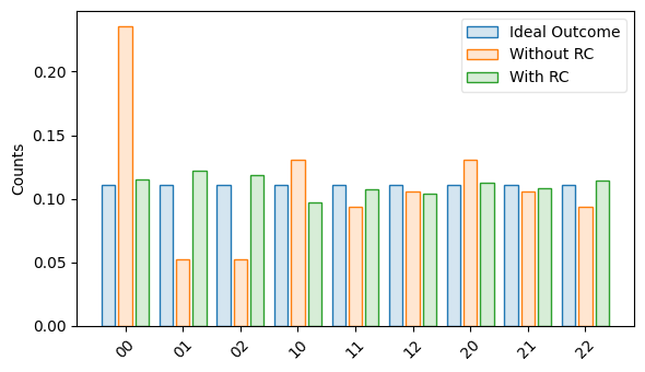
Plot the results:

tq.visualization.plot_results(
    ideal_result,
    noisy_result,
    rc_result,
    labels=["Ideal Outcome", "Without RC", "With RC"],
)

---

Download

Download this file as Jupyter notebook: rc_simple_intro.ipynb.