Selecting Parameters for Error Diagnostics

Due to error processes, quantum states may not evolve according to the expected process. Quantum states can be expressed as a linear combination of observables, and a single processing error may strongly affect some observables while leaving some other observables unaffected.

Most of True-Q™’s error diagnostic protocols rely on the fitting of the exponential decay of one or many observables as a function of circuit length (see [1]). Because the fitting is fundamental to these diagnostic protocols, it is important to understand how to optimally choose the parameters that influence the quality of the fit. This tutorial covers the basic information needed to successfully select values of the arguments that are common for all of True-Q™’s error diagnostic tools:

1. The n_random_cycles argument The n_random_cycles argument tells error diagnostic protocols how many rounds of random cycles to compile into the cycle whose noise is being characterized.

2. The n_circuits argument The n_circuits argument tells True-Q™ how many randomizations of a diagnostic circuit to take for each circuit length specified by n_random_cycles.

The following section gives an introduction to the mathematical modeling of the observables characterized by True-Q™'s error diagnostic protocols.

The n_random_cycles argument

The n_random_cycles argument is used in most of True-Q™’s error diagnostic protocols. It tells the diagnostic protocol how many random cycles to compile into the cycle of interest (or in some cases to append to an empty cycle) when generating circuits used to characterize the noise. This parameter tells True-Q™ where to sample from the exponential decay and can impact the accuracy of the characterization if chosen well or poorly. Below we show two attempts to fit the same decay for different selections of n_random_cycles. In the first image, points are spaced out well on the curve so that the fit is accurate to the shape of the decay. In the second image, the points all fall on the linear part of the decay so the fit is not accurate.

When implementing True-Q™’s diagnostic tools, it is worthwhile to look at the decays to check where the n_random_cycles you have chosen lie on the curve. You can access the decays after populating the results of any error diagnostic CircuitCollection circuits by calling circuits.plot.raw(). As a general rule of thumb, selecting three lengths with the maximum around \(1/p\), where \(p\) is the probability of error, will usually result in a good fit. If the maximum length is too long, more circuits with that length will be needed to accurately characterize the decay.

The n_circuits argument

The n_circuits argument tells True-Q™ how many random samples of circuits to take for each circuit length specified in n_random_cycles. Increasing this parameter will increase the accuracy of the sampled points on the decay being fitted. We set the default value to n_circuits=30 for most of True-Q™’s protocols - this should be sufficient to provide a good estimate in most cases if n_random_cycles is chosen well.

Knowledge of these parameters should be sufficient to get started using True-Q™’s error diagnostic tools, but if you want to explore some more advanced customization options, continue reading in Selecting Parameters for Error Diagnostics (Advanced).

Example

Let’s take a look at how varying these parameters impacts the fit. First, we define a noisy simulator:

import trueq as tq

simulator = tq.Simulator().add_depolarizing(0.03)

Next, we create two circuit collections, one with n_random_cycles=[2, 6], which we expect to result in less accurate estimates of the parameter of interest, and one with a n_random_cycles=[2, 33] to see how the fit differs. Note that the error rate for the above simulator is \(0.03\), and the recommended maximum circuit length in n_random_cycles is then \(1/0.03\approx 33\), so we expect this second choice of n_random_cycles will result in a more accurate fit.

circs_bad_param1 = tq.make_srb(0, n_random_cycles=[2, 6])
circs_good_param = tq.make_srb(0, n_random_cycles=[2, 33])

Now, we run these CircuitCollections on the noisy simulator:

simulator.run(circs_bad_param1)
simulator.run(circs_good_param)

Finally, we look at the fitted parameters for both CircuitCollections.

circs_bad_param1.plot.raw()
circs_good_param.plot.raw()

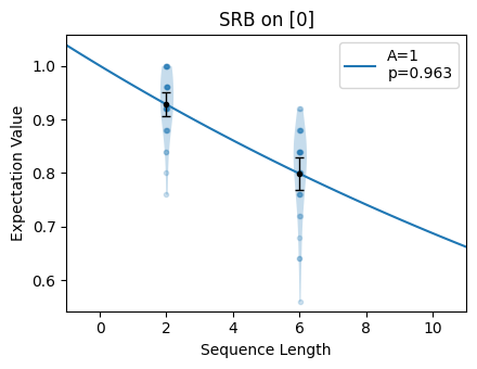
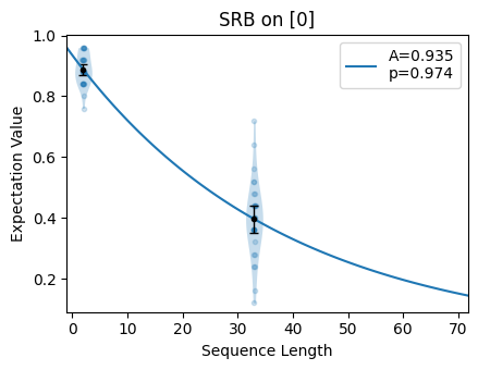
The fitting function for Streamlined Randomized Benchmarking (SRB) returns fit parameters \(p\) and \(A\). The parameter \(p\) gives us information about the error rate we are trying to quantify; the error rate is given by \(1-p\). Notice that for the bad choice of n_random_cycles, the region of the plot where the selected sequence lengths lie is approximately linear. For the good choice of n_random_cycles, the selected sequence lengths span the exponential and the fitted value is more accurate.

Now we will look at the impact of decreasing the n_circuits parameter. Recall that the default value of n_circuits=30 was used to generate circs_good_param. We now generate a CircuitCollection with n_circuits=2:

circs_bad_param2 = tq.make_srb(0, [2, 33], n_circuits=2)

Next we run the new circuit collection and plot the decay curve:

simulator.run(circs_bad_param2)
circs_bad_param2.plot.raw()

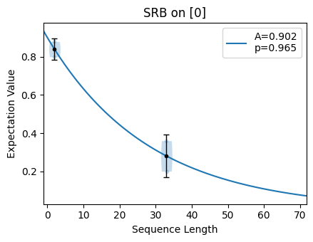
Notice that the error bars on the fit are larger than those for the fit done with good parameters. If we output the fit values for these two scenarios, we can see that the standard deviation (given in the second column) is lower when the fit parameters are chosen well.

circs_good_param.fit()

True-Q formatting will not be loaded without trusting this notebook or rerunning the affected cells. Notebooks can be marked as trusted by clicking "File -> Trust Notebook".

SRB Streamlined Randomized Benchmarking	Cliffords (0,) Key: labels: (0,) protocol: SRB twirl: Cliffords on [0]
${e}_{F}$ The probability of an error acting on the targeted systems during a random gate.	1.9e-02 (1.4e-03) 0.019285396979790065, 0.0014037364421653914
${p}$ Decay parameter of the exponential decay $Ap^m$.	9.7e-01 (1.9e-03) 0.9742861373602799, 0.0018716485895538552
${A}$ SPAM parameter of the exponential decay $Ap^m$.	9.4e-01 (1.1e-02) 0.9354916583675972, 0.011197058846811079

circs_bad_param2.fit()

True-Q formatting will not be loaded without trusting this notebook or rerunning the affected cells. Notebooks can be marked as trusted by clicking "File -> Trust Notebook".

SRB Streamlined Randomized Benchmarking	Cliffords (0,) Key: labels: (0,) protocol: SRB twirl: Cliffords on [0]
${e}_{F}$ The probability of an error acting on the targeted systems during a random gate.	2.6e-02 (6.8e-03) 0.026113870409910422, 0.006763790207792921
${p}$ Decay parameter of the exponential decay $Ap^m$.	9.7e-01 (9.0e-03) 0.9651815061201194, 0.009018386943723896
${A}$ SPAM parameter of the exponential decay $Ap^m$.	9.0e-01 (4.9e-02) 0.9016984071516341, 0.04863644822895653

Mathematical Context

In mathematical terms, an ideal computing process \(\Phi\) (e.g. an ideal quantum circuit) maps an observable \(\rho\) to an observable \(\Phi(\rho)\) whereas the noisy implementation of \(\Phi\), denoted as \(\tilde{\Phi}\), maps the same observable \(\rho\) to a perhaps different observable \(\tilde{\Phi}(\rho)\). Here, we say “perhaps” because some processing errors usually leave some observables invariant.

1. Fidelity

   The extent to which \(\tilde{\Phi}(\rho)\) deviates from the target \(\Phi(\rho)\) can be quantified by their normalized overlap:

   \[f(\rho|\tilde{\Phi}):=\frac{\textrm{Tr}\left[\tilde{\Phi}(\rho)\Phi(\rho)\right]} {\textrm{Tr}\left[\Phi(\rho)\Phi(\rho)\right]},\]

   We refer to this quantity as the fidelity of the observable \(\rho\) given the noisy process \(\tilde{\Phi}\). Here, the denominator only ensures that the fidelity cannot exceed 1. We define the process fidelity \(F_E(\tilde{\Phi})\) as the average of \(f(B_i|\tilde{\Phi})\) over some orthogonal basis \(\{B_i\}\) for \(d \times d\) matrices:

   \[F_E(\tilde{\Phi}):= \frac{1}{d^2}\sum_{B_i \in \{B_i\}} f(B_i|\tilde{\Phi}).\]

   The process fidelity \(F_E\) is used in many of True-Q™'s protocols, including Streamlined Randomized Benchmarking (SRB) and Interleaved Randomized Benchmarking (IRB). The individual \(f(B_i|\tilde{\Phi})\) fidelities are used by several other protocols, including Cycle Benchmarking (CB) and K-body Noise Reconstruction (KNR).

2. Unitarity

   We can quantify the decoherent portion of a noisy process \(\tilde{\Phi}\) by looking at how much it contracts the Bloch space. More formally, if we look at a traceless operator \(\rho\), we can use its squared contraction ratio under the action of the noisy process \(\tilde{\Phi}\) to quantify the decoherence of the channel:

   \[\upsilon(\rho|\tilde{\Phi}):=\frac{\textrm{Tr}\left[\tilde{\Phi}(\rho)\tilde{\Phi}(\rho)\right]} {\textrm{Tr}\left[\Phi(\rho)\Phi(\rho)\right]} = \left(\frac{\|\tilde{\Phi}(\rho)\|_2}{\|\rho\|_2}\right)^2.\]

   We can define the unitarity of a channel as an average of the above ratio over an orthonormal basis \(\mathbb{B}\) which contains the identity:

   \[u(\tilde{\Phi}):=\frac{1}{d^2-1}\sum_{B_i\in\mathbb{B}\backslash I} \upsilon(B_i|\tilde{\Phi}).\]

   Equivalently, we can define the unitarity as the average of \(\upsilon(|\psi \rangle \langle \psi|-\mathbb{I_d}/d|\tilde{\Phi})\) over pure states \(|\psi \rangle\) sampled uniformly according to the Haar measure:

   \[u(\tilde{\Phi}):=\mathbb E_{\rm Haar} \upsilon(|\psi \rangle \langle \psi|-\mathbb{I_d}/d|\tilde{\Phi}).\]

   The unitarity is \(1\) when the errors are purely coherent in nature, and is the parameter of interest returned by Extended Randomized Benchmarking (XRB).

As noisy quantum circuits increase in length, the process fidelity and unitarity of most observables in the expansion of the quantum state decay exponentially. The error diagnostic protocols which quantify the parameters introduced above therefore rely on fitting either an exponential decay or a sum of exponential decays.