---

Download

Download this file as Jupyter notebook: leakage.ipynb.

Example: Simulating Leakage

The simulator is capable of adding extra energy levels to allow noise models that include leakage. For example, if a circuit acts on qubits, so that gates are either 2-by-2 for single qubit gates and 4-by-4 for two-qubit gates, then one can direct the simulator to add an extra energy level to each qubit, so that each subsystem is simulated with 3 dimensions. Noise models can interact with the extra level(s).

Extra leakage dimensions are added by the simulator whenever some noise source explicitly asks for a specific dimension. Certain noise sources, such as overrotation, work no matter how many extra levels are included.

import trueq as tq
import trueq.simulation as tqs
import numpy as np
import scipy.linalg as la

Kraus Noise

The most versatile method of adding leakage is through Kraus operator noise with the add_kraus() method. Recall that Kraus noise is specified as a set of operators \(\{K_i\}_{i=1}^m\) and acts on a given density matrix as \(\rho\mapsto\sum_{i=1}^m K_i\rho K_i^\dagger\). To add leakage to a model, we construct Kraus operators with a dimension strictly bigger than the dimension of our gates, and add terms that cause population transfer into these new levels, either stochastically or coherently. The increased dimension must be specified using the dim argument of the add_kraus() method.

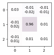
In the following toy example, we add Kraus operators that add no noise with 95% probability, but apply a random (but fixed) qutrit unitary with probability 5%. This induces a stochastic population transfer into the leakage level.

p = 0.05
sim = tq.Simulator()
sim.add_kraus(
    [np.sqrt(1 - p) * np.eye(3), np.sqrt(p) * tq.math.random_unitary(3)], dim=3
)
circuit = tq.Circuit([{0: tq.Gate.x}])
tq.plot_mat(sim.state(circuit).mat())

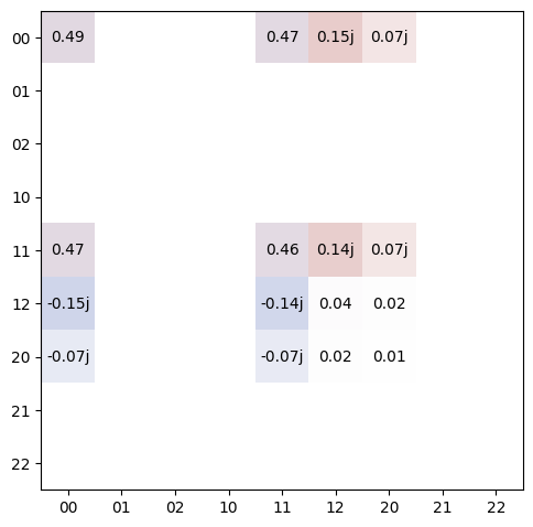
In the next example, we add a coherent leakage term to a CNOT gate with the transitions \(|00\rangle\leftrightarrow|20\rangle\) and \(|10\rangle\leftrightarrow|12\rangle\) that occur at different rates.

sim = tq.Simulator()
ham = np.zeros((9, 9), dtype=np.complex128)
ham[([0, 6], [6, 0])] = 0.5
ham[([3, 5], [5, 3])] = 1

ops = la.expm(-1j * 0.3 * ham)
sim.add_kraus([ops], match=tqs.GateMatch(tq.Gate.cnot), dim=3)
circuit = tq.Circuit([{0: tq.Gate.h}, {(0, 1): tq.Gate.cx}])
tq.plot_mat(sim.state(circuit).mat(), xlabels=3, ylabels=3)

Measurement Classification

In the first example, we add asymmetric classification error to all three levels, where a \(|0\rangle\) is reported as a ‘0’ 99% of the time, a \(|1\rangle\) is reported as a ‘1’ 92% of the time, and a \(|2\rangle\) is reported as a ‘2’ 80% of the time. Off-diagonals are the probabilities of misclassification into specific outcomes corresponding to the row they are located in. We do this by using the add_readout_error() simulator method that supports confusion matrix inputs.

# define a confusion matrix for a qutrit
confusion = [[0.99, 0.03, 0.02], [0.005, 0.92, 0.18], [0.005, 0.05, 0.8]]

# simulate the effects on all three basis states
circuit = tq.Circuit([{0: tq.Prep()}, {0: tq.Meas()}])
for idx, prep_state in enumerate(np.eye(3)):
    sim = tq.Simulator().add_readout_error(errors={0: confusion}).add_prep(prep_state)
    sim.run(circuit, n_shots=np.inf, overwrite=True)
    print(f"Prepare |{idx}>:", circuit.results)

Prepare |0>: Results({'0': 0.99, '1': 0.005, '2': 0.005}, dim=3)
Prepare |1>: Results({'0': 0.03, '1': 0.92, '2': 0.05}, dim=3)
Prepare |2>: Results({'0': 0.02, '1': 0.18, '2': 0.8}, dim=3)

In the next example, we simulate with a qutrit, but we only classify into bits. This situation arises, for example, in superconducting qubits when there is leakage into the third level of the anharmonic oscillator, but readout always reports a ‘0’ or a ‘1’. We achieve this by defining a rectangular confusion matrix where \(|2\rangle\) is classified as a ‘0’ 70% of the time, and as a ‘1’ 30% of the time. Additionally, \(|0\rangle\) and \(|1\rangle\) also have their own classification errors, too.

confusion = [[0.99, 0.08, 0.7], [0.01, 0.92, 0.3]]

# simulate the effects on all three basis states
circuit = tq.Circuit([{0: tq.Prep()}, {0: tq.Meas()}])
for idx, prep_state in enumerate(np.eye(3)):
    sim = tq.Simulator().add_readout_error(errors={0: confusion}).add_prep(prep_state)
    sim.run(circuit, n_shots=np.inf, overwrite=True)
    print(f"Prepare |{idx}>:", circuit.results)

Prepare |0>: Results({'0': 0.99, '1': 0.01})
Prepare |1>: Results({'0': 0.08, '1': 0.92})
Prepare |2>: Results({'0': 0.7, '1': 0.3})

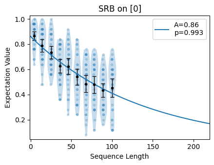
We can see the effect that this has on a 1-qubit benchmarking experiment. Here, we add gate noise that stochastically populates the third level with probability 1% every time a gate is applied.

p = 0.01
perm02 = np.array([[0, 0, 1], [0, 1, 0], [1, 0, 0]])
perm12 = np.array([[1, 0, 0], [0, 0, 1], [0, 1, 0]])
sim.add_kraus(
    [np.sqrt(1 - p) * np.eye(3), np.sqrt(p / 2) * perm02, np.sqrt(p / 2) * perm12],
    dim=3,
)
circuits = tq.make_srb(0, np.linspace(4, 100, 10).astype(int))
sim.run(circuits)
circuits.plot.raw()

---

Download

Download this file as Jupyter notebook: leakage.ipynb.